Measuring Cloud Oktas from Outer Space
This article describes the approach undertaken by data scientists at Axibase to calculate cloud cover using satellite imagery from the Japanese Himawari 8 satellite.
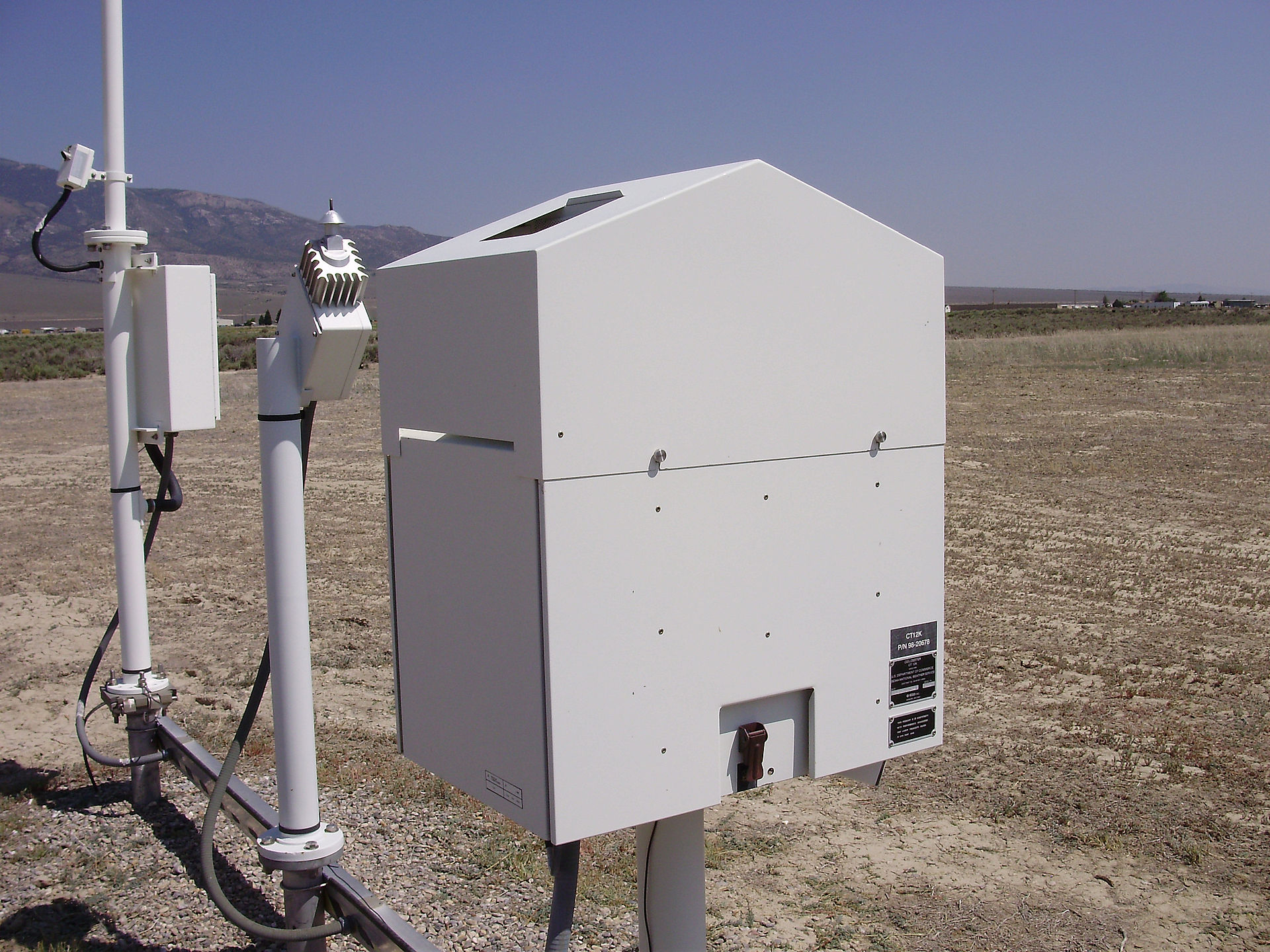
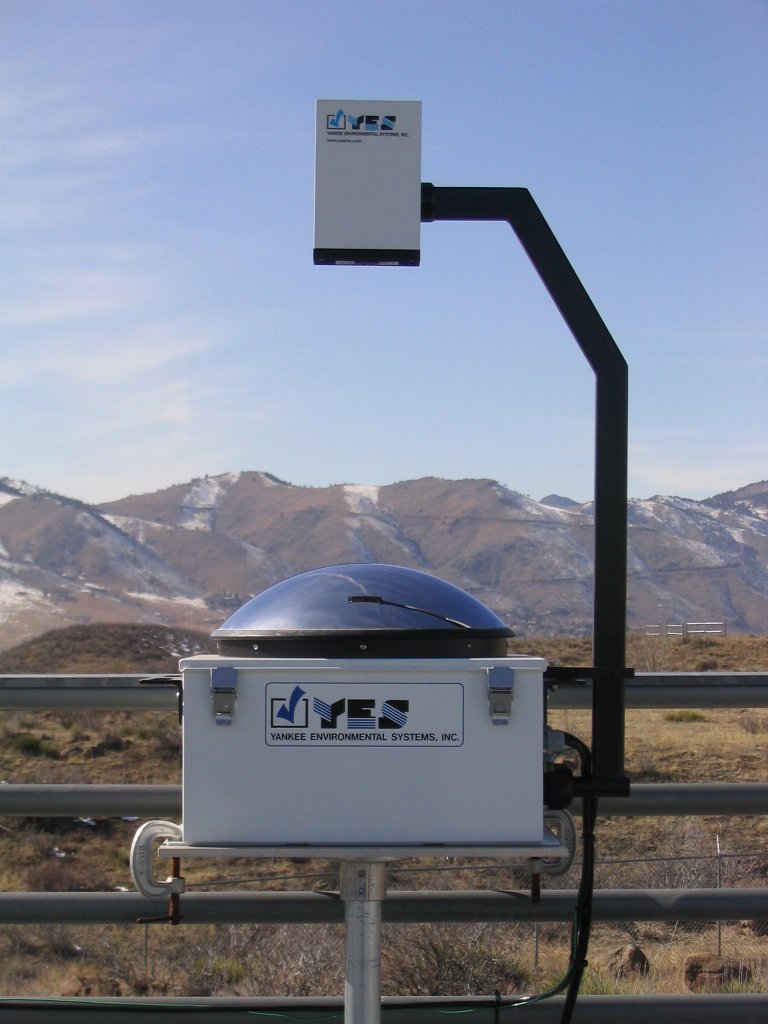
Today, cloud cover is measured using automated weather stations, specifically ceilometers and sky imager instruments. The ceilometer is an upward pointed laser that calculates the time required for the laser to reflect back to ground surface from overhead clouds, which determines the height of the cloud base. The sky imager divides the sky into regions and finds the percentage of clouds in those different regions. Only clouds located directly overhead are detected. As a result, with how sparsely weather stations are placed today, the amount of cloud cover data is limited. Most modern weather stations can discover and measure clouds up to a ceiling of 7600 meters. You can learn more about modern automated weather stations and ceilometers on Wikipedia.
Ceilometer:
Sky Imager:
You can learn more about automated weather stations in Australia on the official website of the Bureau of Meteorology Australia.
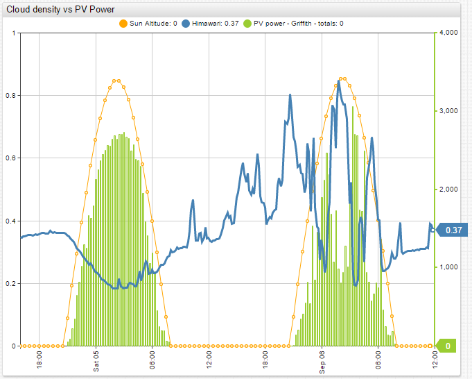
Cloud cover measurements have many applications and benefits in weather forecasting and solar energy generation. For example, seasonal cloud cover statistics allow tourists to plan their holidays for sunnier weeks and months of the year. This information is also useful to mountain climbers planning their ascent, since they need to choose seasons with less cloud cover, guaranteeing the best possible conditions for their summit attempts. Photovoltaic energy generation hinges heavily on quality cloud cover data. Solar panels are most efficient when there are no clouds, so when building a solar power station it is important to analyze cloud oktas data. Because automated weather stations that measure this metric are distributed sparsely, the data is often not available. Below is a visualization comparing cloud cover with solar power generation for a particular station in Australia. It is readily apparent that the two metrics are interdependent.
This research project is aimed at calculating cloudiness over Australia from satellite images. Our goal is to use a simple method that can effectively determine the cloud cover without employing complex algorithms and machine learning. We compared our results with actual data from ground weather stations. Using data available from the JMA (Japan Meteorological Agency) and the Australian BOM (Bureau of Meteorology) made this research especially interesting and feasible.
Cloudiness Data
Australian meteorological stations are used as the source of cloudiness data. The list of all meteorological stations is available on the website of the Australian Bureau of Meteorology.
Here is a summary of the available stations:
- 20112 – total number of meteorological stations.
- 7568 – total number of currently functional stations.
- 867 – total number of station that have available data.
- 778 – total number of station whose data is loaded into ATSD.
- 394 – total number of stations that measure cloud_oktas.
- 45 – total number of station that measure cloud oktas at least 4 times per day.
Cloud cover measurements are available from the Australian Bureau of Meteorology Latest Weather Observations portal. Each station’s cloud cover data for the past few days can be retrieved in JSON format using the REST API.
As stated on Wikipedia, cloud cover is the fraction of the sky obscured by clouds when observed from a particular location. It is measured in “oktas” (meaning “eighths”): 0, 1/8, 2/8, …, 1. Several methods are used to measure cloud cover and it is not exactly clear which of them is used by the Australian weather stations.
Satellite Data
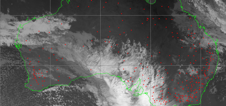
We analyzed images from a Japanese geostationary weather satellite, Himawari 8. The launch of this satellite took place on October 7, 2014 and it became operational on July 7, 2015. It provides high quality images of the Earth in 16 frequency bands every 10 minutes. You can learn more about Himawari satellites and imaging on the Meteorological Satellite Center of JMA website.
The Japan Meteorological Agency (JMA) processes the satellite images and determines several parameters of the clouds. The results can viewed on the Meteorological Satellite Center of JMA website.
The algorithms used by JMA to process the images are complex. Read this article to learn more about their algorithms.
To determine cloud cover from Himawari images as simply as possible, we analyzed only one of the bands. For this research project, we used images of Australia available from the MSC JMA Real Time Image portal. The server keeps images for the past 24 hours. We decided to use images in infrared band 13 with wavelength equal to 10400 nm.
Data Flow
We used the Axibase Time Series Database to collect data from the Australian Bureau of Meteorology in JSON format. ATSD comes with the Axibase Collector, which collects data from any remote source and stores it in ATSD. Another benefit of ATSD was the built-in visualization that allowed us to graph our results, giving us a good understanding of our progress.
The images from JMA are loaded in PNG format into R, where they are analyzed. To analyze the images in R, we used the EBImage, oce, and geosphere R packages. The results of the analysis are stored in ATSD.
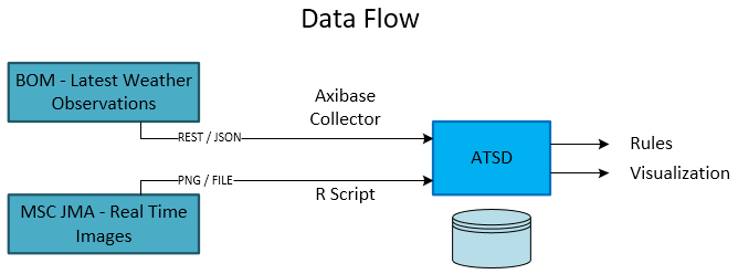
Once both the actual cloud oktas and the calculated cloud oktas were loaded into ATSD, visualization portals were built to compare the collected and computed metrics.
Cloudiness Detection From Images
Using the geographical coordinates of each station, we determined each station’s location on the satellite images. The images are somewhat distorted near the border of Australia and on the lines of the coordinate grid. This distortion comes in the form of overlays added on top of the images, the green Australian border and white grid. Therefore, we only studied stations that are far from the distorted areas.
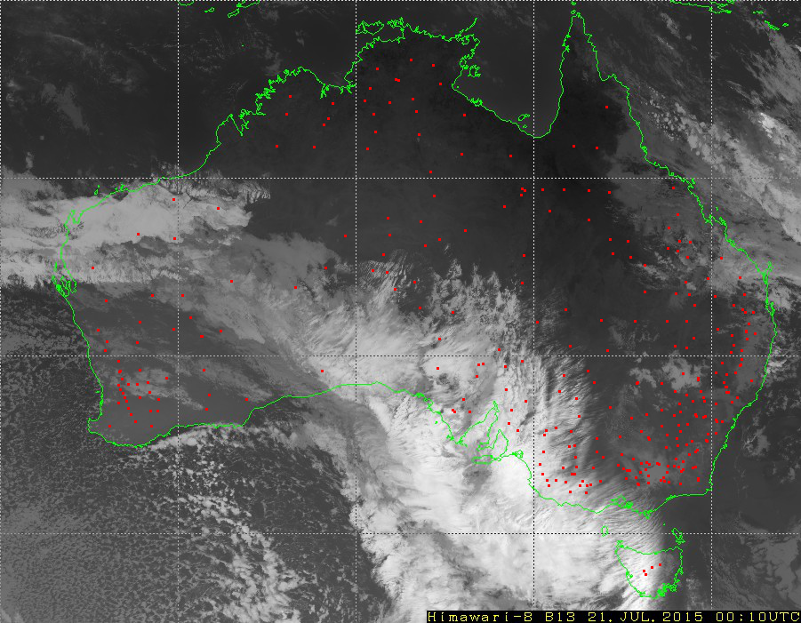
We used a simple method to detect clouds. Since clouds are cooler than the earth’s surface, they will be rendered white on the satellite images, and the earth’s surface w black. Therefore, the brightness of the pixels in the images reflects cloudiness. Hence, we calculated cloud cover for a given meteorological station as the average pixel brightness over a 3 * 3 square of pixels, centered over the station.
Since one pixel on the image, depending on the location, covers an area from 5.5 * 3.9 to 5.5 * 5.6 square kilometers, it turns out that for the determination of cloudiness we analyzed an area of about 230 square kilometers.
Here is the key line from the R script used to calculate the cloudiness_himawari_b13 metric from the satellite images:
To store the results in ATSD, the following code is used:
Once we stored the calculation results in ATSD, we were able to view graphs of actual and calculated cloud cover in Axibase Chart Lab. For example, here is a Chart Lab portal for the weather station near the town of Oakey:
In this Chart Lab portal the cloudiness_himawari_b13 metric is the calculated cloud cover, and the cloud_oktas metric is cloud cover measured by the station.
We selected stations that measure cloud cover at an average frequency of at least once every 4 hours. The table below displays the Pearson correlation coefficient between actual and calculated cloud cover for the selected stations:
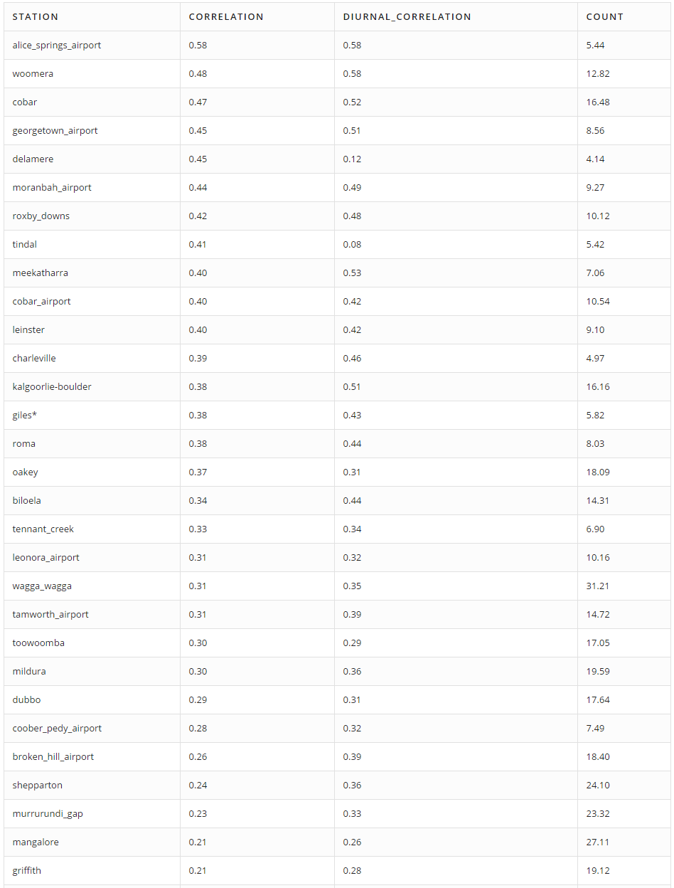
NOTE: the Count column indicates the average number of cloud cover measurements per day.
In conclusion, the selected approach does not appear to work particularly well and there is little correlation between computed and factual values.
Interestingly, the cloudiness_himawari_b13 series has a daily cycle; it is less during the day than at night. We clearly see this trend if we compare this series with the height of the sun above the horizon (sun altitude). Sun altitude is calculated using a script created by Vladimir Agafonkin.
The results clearly show that the correlation during daytime hours is somewhat higher.
We tried to remove the diurnal cycle by subtracting the average of values of the last n days. Here are the results with the diurnal cycle removed:
Improving the Correlation
We attempted to improve the correlation by adjusting the method for determining the cloudiness from an image.
We made the following adjustments:
- We averaged out the brightness over different areas of the images.
- We took a weighted average of brightness over large areas of the image, giving less weight to pixels more distant from the center of the area. To calculate the weights, we used geometrical principles, as described below. We took into account the height of the cloud’s lower edge directly over a station. Meteorological stations measure the height of clouds and this data is available from the Australian Bureau of Meteorology. It seems that the lower the height of the cloud the greater the value of cloud cover.
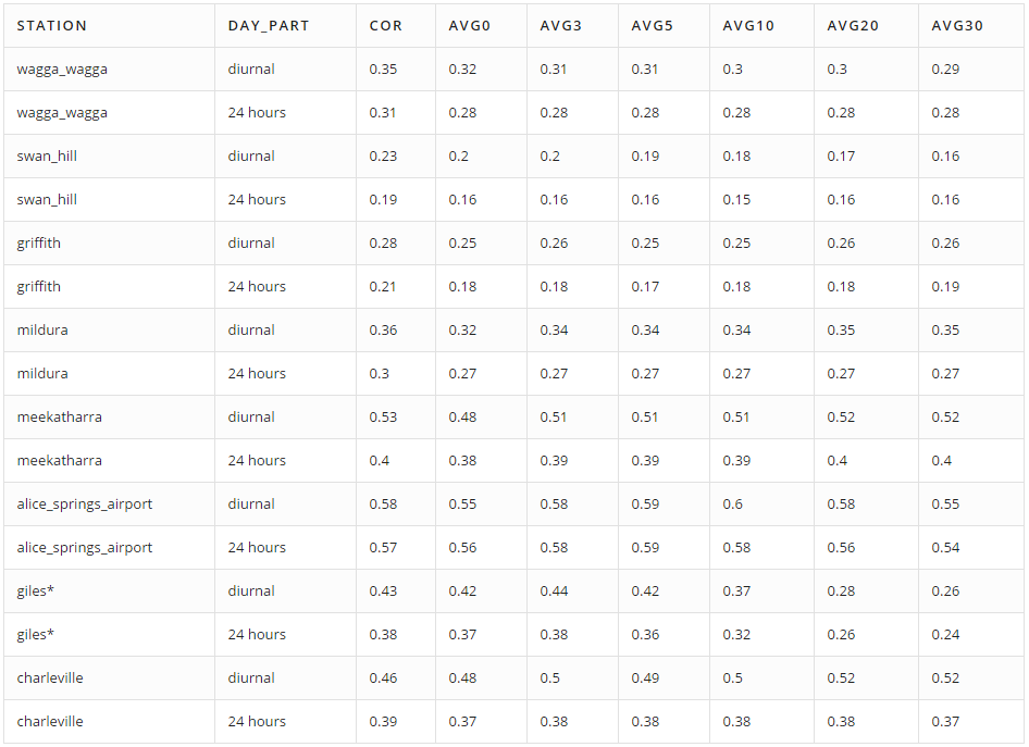
To be more concrete, here are example computations for 8 meteorological stations. We choose them because they have enough measurements of cloud cover and are far from the overlaid white lines on the images.
For each of the stations we selected 5 disks (they are not perfectly round) with radii of 0, 3, 5, 10, 20, 30 pixels:


Averaged brightness over each disc is an estimation of the cloud cover. So we have 6 estimations, and their correlations with actual values of cloud cover are saved in columns avg0, …, avg30 in the following tables:
Averaged Brightness:
Weighted Average Brightness:
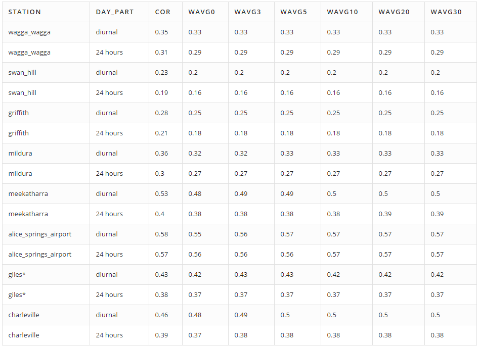
Columns wavg0, … wavg30 display correlations between cloud cover and the weighted average of brightness for given disks. To compute the weight (w) of each pixel, we use the following equation:
$w = \frac{h}{(d^2 + h^2)^{3/2}} = \frac{h}{l^3}.$
In this equation, d is the distance between the center of the pixel and the given station (in meters) and h is the cloud height (in meters). So distant and high clouds have lower weights.
Here is a code snippet from the R script that we used to calculate the weighted average of brightness for given disks:
Unfortunately, since we know only the height of the clouds directly above each station, we use this height when calculating the weighted average for all pixels, assuming that the height of all clouds is the same around each station.
To explain the reasoning behind using this formula, let’s assume that clouds are flat (this assumption is incorrect, but we will use it anyways). A flat cloud with an area of A squared meters has height of h meters above the ground and is d meters away of station. As a result, the “solid angle” of the cloud for the station is approximately equal wA:
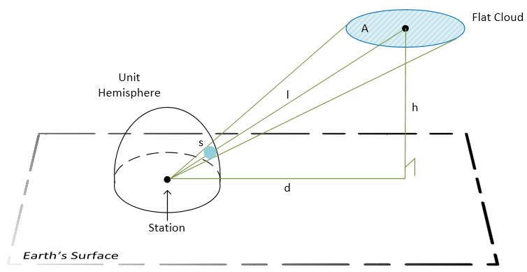
Legend:
- A – the cloud area.
- h – the height of the cloud.
- d – distance from the station to the center of the cloud’s projection on the ground.
- l – distance between the station and the center of the cloud.
- s – the area of the cloud’s image on the unit hemisphere. This tells us how big the cloud appears to the station.
$s = \int_A w\ d\sigma \approx w\cdot A$, where $w = \frac{h}{(d^2 + h^2)^{3/2}} = \frac{h}{l^3}.$
The measurement of a “solid angle” is equal to the area of intersection of this angle and the unit sphere centered in the angle vertex. So the contribution of a pixel to cloud cover is proportional to the w coefficient, because all pixels on an image cover nearly the same area equal to A. The exact statement is that the integral of w over the area A equals to the “solid angle.”
The results show that none of the methods used to improve the correlation led to a significant increase.
Changing the Original Logic – Improved Correlation
To improve the correlation, we decided to change the original logic of how cloud oktas are determined from satellite images. Rather than using black as the earth’s color, we determined a shade of grey (for each station) that the earth (without cloud cover) reached during the day and used it as the base of our calculations. This logic was used because the temperature of the earth’s surface changes during the day, meaning that its brightness on the satellite images changes as well. The brightest point occurred during the night, when the earth is at its coolest. All darker shades are considered cloudless, and lighter shades are considered cloudy.
This approach lead to an improvement in correlations. This approach also decreased the diurnal cycle.
Here are the calculations and results for the town of Oakey:
The lower brightness threshold = 0.2916667.
All values below the lower threshold are zeroed out.
The upper brightness threshold = 0.4583333.
All values are scaled – divided by the upper brightness threshold.
Those values greater than 1 are set equal to 1.
Conclusion
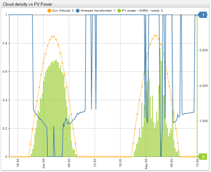
When comparing the calculated cloud oktas with solar power generation for a particular station, it is clear that this algorithm can be used as a basis of forecasting and power generation planning.
The above Chart Lab portal compares the power generation of a solar power station near one of the automated weather stations in the city of Griffith, for which we calculated cloud cover. The solar power station is 3 kilometers away from the automated weather station. From these results it is clear that increases in calculated cloud cover lead to decreases in solar power generation and vice-versa. This means that there is a correlation between the calculated cloud oktas and solar power generation.
If we compare the improved correlation results with solar power generation for the same station, their interdependency is even more apparent. There is a strong correlation between the improved calculated cloud cover and solar power generation.
The results of this research project lead us to believe that our algorithm can be used as a way to calculate cloud oktas with relative accuracy. The calculated cloud cover accuracy is high enough that it can be used to forecast and plan solar energy production. This conclusion is especially true for areas that are not covered by BOM meteorological weather stations, where there is no other real source of cloud cover data.