Cell References in SQL and Excel

Overview

This article contains examples of how analytic functions in SQL can be used to emulate step-by-step calculations in Microsoft Excel.

Staged Calculations in Excel

To assist users in organizing complex analysis into step-by-step calculations, Excel provides a convenient A1 addressing notation, or reference style, to pass calculation results between cells by value:

Columns are assigned letter names, starting with A for the left-most column.
Rows are assigned ordinal numbers, starting with 1 for the top row.
=B2 returns the value of cell located in column B and row 2.
=B3 - B2 returns the difference between values of cells B3 and B2.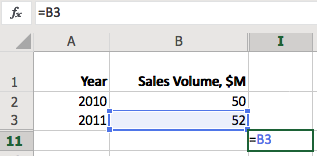

Users can calculate the year-on-year change by entering =B3 - B2 formula as the value of the current cell.

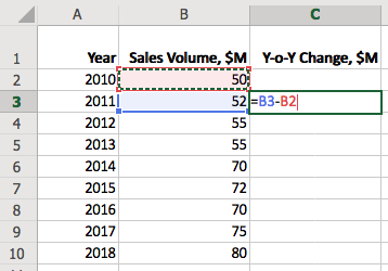
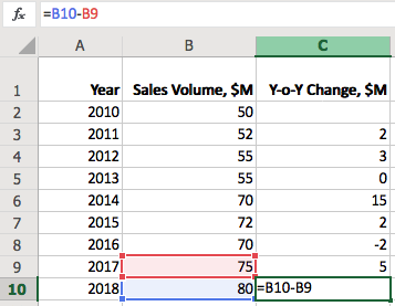
Such references are relative, and the row index is updated behind the scenes when you copy the cell to fill the Y-o-Y Change, $M column.

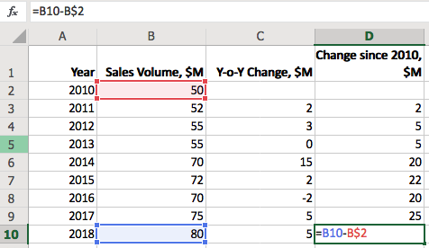
To fix the row in the address, use $ prefix, for example =B3 - B$2. This makes it possible to calculate change in sales since 2010, for example.

Analytic Functions in SQL

To achieve the same results in SQL we need to first cover a special class of functions called analytic functions.

The analytic functions in SQL allow access to grouped statistics without reducing the number of rows returned by the query.

SELECT value,
  -- SUM(value) below is calculated without GROUP BY
  value/SUM(value) OVER() AS weight
FROM table-name ORDER BY weight DESC

Often called windowing functions due to their ability to operate on ordered and partitioned groups of records, analytic functions are different from aggregate functions which reduce multiple rows in the same group into a single result row.

Many aggregate functions such as SUM, AVG, and COUNT can be invoked as analytic functions using the OVER clause. However the class of analytic functions also includes reference functions which operate on an ordered set of records. Such reference functions include:

LAG. Provides access to a previous row at a specified offset from the current position.
LEAD. Provides access to a following row at a specified offset from the current position.
FIRST_VALUE. Provides access to the first row.
LAST_VALUE. Provides access to the last row.

Documentation Links

Excel cell referencing
ATSD LAG function
Oracle LAG function

Referencing in SQL

The purpose of the LAG and LEAD functions in SQL is similar - to access a column value in a preceding or following row.

Assuming the same dataset is loaded in the database, it can be queried with a SELECT statement as follows:

SELECT date_format(time, 'yyyy') AS "Year",
  value AS "Sales Volume, $M"
FROM "win-sales"
  ORDER BY time

| Year | Sales Volume, $M |
|------|------------------|
| 2010 |               50 |
| 2011 |               52 |
| 2012 |               55 |
| 2013 |               55 |
| 2014 |               70 |
| 2015 |               72 |
| 2016 |               70 |
| 2017 |               75 |
| 2018 |               80 |

Relative References

Similar to Excel, the reference in LAG function consists of the column name and the row offset, which starts with 1 by default. Excel assigns column names automatically, starting with A (up to 16,384 are allowed). In SQL, the function must to refer to the name of an existing column or alias such as LAG(value).

SELECT date_format(time, 'yyyy') AS "Year",
  value AS "Sales Volume, $M",
  LAG(value) AS "Previous Sales Volume, $M",
  value - LAG(value) AS "Y-o-Y Change, $M"
FROM "win-sales"

| Year | Sales Volume, $M | Previous Sales Volume, $M | Y-o-Y Change, $M |
|------|------------------|---------------------------|------------------|
| 2010 |               50 |                           |                  |
| 2011 |               52 |                        50 |                2 |
| 2012 |               55 |                        52 |                3 |
| 2013 |               55 |                        55 |                0 |
| 2014 |               70 |                        55 |               15 |
| 2015 |               72 |                        70 |                2 |
| 2016 |               70 |                        72 |               -2 |
| 2017 |               75 |                        70 |                5 |
| 2018 |               80 |                        75 |                5 |

The value - LAG(value) expression returns the same results as =B3 - B2 in Excel. In this case B and value are equivalent column names.

To accomplish the same result in Oracle Database, add OVER clause after each analytical function.

Oracle SQL version:

SELECT time AS "Year",
  value AS "Sales Volume, $M",
  LAG(value) OVER (ORDER BY time) AS "Previous Sales Volume, $M",
  value - LAG(value) OVER (ORDER BY time) AS "Y-o-Y Change, $M"
FROM win_sales

Absolute References

FIRST and LAST functions can be used to access first and last rows in the partition respectively. This is equivalent to =B3 - B$2 in Excel which calculates the change in sales since 2010.

SELECT date_format(time, 'yyyy') AS "Year",
  value AS "Sales Volume, $M",
  LAG(value) AS "Previous Sales Volume, $M",
  value - LAG(value) AS "Y-o-Y Change, $M",
  value - FIRST_VALUE(value) AS "Change since 2010, $M"
FROM "win-sales"
  WITH ROW_NUMBER(entity, tags ORDER BY time) > 0

| Year | Sales Volume, $M | Previous Sales Volume, $M | Y-o-Y Change, $M | Change since 2010, $M |
|------|------------------|---------------------------|------------------|-----------------------|
| 2010 |               50 |                         0 |                0 |                     0 |
| 2011 |               52 |                        50 |                2 |                     2 |
| 2012 |               55 |                        52 |                3 |                     5 |
| 2013 |               55 |                        55 |                0 |                     5 |
| 2014 |               70 |                        55 |               15 |                    20 |
| 2015 |               72 |                        70 |                2 |                    22 |
| 2016 |               70 |                        72 |               -2 |                    20 |
| 2017 |               75 |                        70 |                5 |                    25 |
| 2018 |               80 |                        75 |                5 |                    30 |

Oracle SQL version:

SELECT time AS "Year",
  value AS "Sales Volume, $M",
  LAG(value) OVER (ORDER BY time) AS "Previous Sales Volume, $M",
  value - LAG(value) OVER (ORDER BY time) AS "Y-o-Y Change, $M",
  value - FIRST_VALUE(value) OVER (ORDER BY time) AS "Change since 2010, $M"
FROM win_sales

Aggregate Functions

Sliding Total

To calculate a running (sliding) total in Excel, one can pass a relative range of cell values, for example: =SUM(B2:B4).

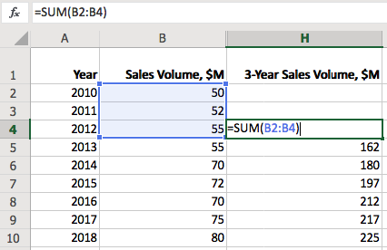
To return the same result in SQL one can add LAG results with increasing offsets.

SELECT date_format(time, 'yyyy') AS "Year",
  value AS "Sales Volume, $M",
  value + LAG(value) + LAG(value,2) AS "3-Year Sales Volume, $M"
FROM "win-sales"

| Year | Sales Volume, $M | 3-Year Sales Volume, $M |
|------|------------------|-------------------------|
| 2010 |               50 |                         |
| 2011 |               52 |                         |
| 2012 |               55 |                     157 |
| 2013 |               55 |                     162 |
| 2014 |               70 |                     180 |
| 2015 |               72 |                     197 |
| 2016 |               70 |                     212 |
| 2017 |               75 |                     217 |
| 2018 |               80 |                     225 |

Oracle SQL version:

SELECT time AS "Year",
  value AS "Sales Volume, $M",
  value + LAG(value) OVER (ORDER BY time) + LAG(value,2) OVER (ORDER BY time) AS "3-Year Sales Volume, $M"
FROM win_sales

However, if the number of rows is large enough, applying an aggregate function to all values within the fixed-length partition is more efficient.

SELECT date_format(time, 'yyyy') AS "Year",
  value AS "Sales Volume, $M",
  SUM(value) AS "3-Year Sales Volume, $M"
FROM "win-sales"
  WITH ROW_NUMBER(entity, tags ORDER BY time) <= 3

The above query produces the same result using the SUM function with the size of the sliding window controlled in the ROW_NUMBER clause.

Oracle version:

SELECT time AS "Year",
  value AS "Sales Volume, $M",
  SUM(value) OVER(ORDER BY time ROWS BETWEEN 2 PRECEDING AND CURRENT ROW) AS "3-Year Sales Volume, $M"
FROM win_sales

Growing Total

To calculate a growing total in Excel, set the starting row to an absolute value =SUM(B$2:B4).

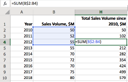
To calculate a growing total for all values in the column in SQL, create a single partition ordered by time and disable row filtering with ROW_NUMBER > 0.

SELECT date_format(time, 'yyyy') AS "Year",
  value AS "Sales Volume, $M",
  SUM(value) AS "Total Volume since 2010, $M"
FROM "win-sales"
  WITH ROW_NUMBER(entity, tags ORDER BY time) > 0

| Year | Sales Volume, $M | Total Volume since 2010, $M |
|------|------------------|-----------------------------|
| 2010 |               50 |                          50 |
| 2011 |               52 |                         102 |
| 2012 |               55 |                         157 |
| 2013 |               55 |                         212 |
| 2014 |               70 |                         282 |
| 2015 |               72 |                         354 |
| 2016 |               70 |                         424 |
| 2017 |               75 |                         499 |
| 2018 |               80 |                         579 |

Oracle SQL version:

SELECT time AS "Year",
  value AS "Sales Volume, $M",
  SUM(value) OVER (ORDER BY time) AS "Total Volume since 2010, $M"
FROM win_sales

Appendix: Sample Dataset

ATSD data commands

series e:win-test d:2010-01-01T00:00:00Z m:win-sales=50
series e:win-test d:2011-01-01T00:00:00Z m:win-sales=52
series e:win-test d:2012-01-01T00:00:00Z m:win-sales=55
series e:win-test d:2013-01-01T00:00:00Z m:win-sales=55
series e:win-test d:2014-01-01T00:00:00Z m:win-sales=70
series e:win-test d:2015-01-01T00:00:00Z m:win-sales=72
series e:win-test d:2016-01-01T00:00:00Z m:win-sales=70
series e:win-test d:2017-01-01T00:00:00Z m:win-sales=75
series e:win-test d:2018-01-01T00:00:00Z m:win-sales=80

Oracle SQL:

CREATE TABLE win_sales (
 time int,
 value NUMBER
)

INSERT INTO win_sales (time, value) VALUES (2010, 50);
INSERT INTO win_sales (time, value) VALUES (2011, 52);
INSERT INTO win_sales (time, value) VALUES (2012, 55);
INSERT INTO win_sales (time, value) VALUES (2013, 55);
INSERT INTO win_sales (time, value) VALUES (2014, 70);
INSERT INTO win_sales (time, value) VALUES (2015, 72);
INSERT INTO win_sales (time, value) VALUES (2016, 70);
INSERT INTO win_sales (time, value) VALUES (2017, 75);
INSERT INTO win_sales (time, value) VALUES (2018, 80);

# Cell References in SQL and Excel

# Overview

# Staged Calculations in Excel

# Analytic Functions in SQL

# Documentation Links

# Referencing in SQL

# Relative References

# Absolute References

# Aggregate Functions

# Sliding Total

# Growing Total

# Appendix: Sample Dataset