# Violence Begets Violence: An Analysis of the Baltimore Police Force and Baltimore Homicide Data

# Methodology

The City of Baltimore, Maryland has published data about incidents of force used by the Police Department which have come under investigation by the BPD Force Investigation Team. Using this data set, which begins in 2013 and continues until the end of 2015, these actions can be scrutinized based on a number of criteria including the location of the incident, the nature of the incident, and the date of the incident.

Additionally, the City of Baltimore has recorded crime incidents in the city, including homicide rates during the years 2013 and 2014. Baltimore has one of the highest murder rates in the country, and even ranks 19th on the planet for highest per capita murder rate. These two data sets can be compared and contrasted to underline a number of features regarding the nature and the scope of the violence that occurs against the backdrop of a nearly three hundred year old city less than forty miles from the Washington, DC.

To establish a correlation between incidents of police use of force and incidents of homicide, it must be possible to effectively predict the occurrence of an above average amount of incidents of police use of force using data about the number of homicides that occurred in a given neighborhood. To establish a standard, for the sake of testing, mean values from each dataset are collected. This mean is compared to observed data from each dataset, and if a district is found to have witnessed an above average number of murders during the observed period, the alternative hypothesis predicts that the district also sees an above average number of incidents of police use of force.

Both of these datasets can be analyzed in the Axibase Time Series Database (ATSD) which provides a built-in support for the Socrata Open Data format used by the majority of government agencies in the United States. ATSD also includes graphics capabilities to analyze the data with SQL and visualize it with graphs.

For information about performing these steps in your own ATSD instance, see the Action Items section below.

# Data

The general format for SQL queries for this dataset is:

SELECT tags.$TAG_NAME$, count(*), datetime
  FROM "row_number.3w4d-kckv"
GROUP BY tags.$TAG_NAME$, PERIOD(1 MONTH)
  ORDER BY tags.$TAG_NAME$, datetime

The $TAG_NAME$ represents one of the dimensions of the time series collected within the dataset, such AS "district", while 3w4d-kckv represents the unique identifier of the dataset in the data.gov catalog.

The SQL syntax allows the user to ask and answer a series of relevant questions about both sets of data, and ChartLab allow the user to visualize and compare this data for a deeper understanding of the information.

# Location of Homicides

Organize the data considering the location of the homicide:

SELECT tags.district, count(*)
  FROM "row_number.3w4d-kckv"
GROUP BY tags.district
  ORDER BY tags.district

Notice the time period is not set to calculate the break-down of police use of force incidents for the entire timespan.

This results of this query are as follows:

| tags.district | count(*) |
|---------------|----------|
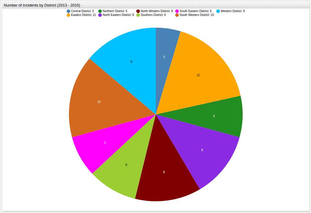
| null          | 3        |
| CD            | 3        |
| ED            | 11       |
| ND            | 5        |
| NED           | 8        |
| NWD           | 8        |
| SD            | 6        |
| SED           | 5        |
| SWD           | 10       |
| WD            | 9        |

The data has been sorted by district whose names correspond to the Baltimore City Planning Map shown below. Data lacking location information has been displayed with the district tag null. Notice that the Eastern District of the city is split into two Police Precincts (Eastern and Southeastern), and the unlabeled blue area just below the Central District is considered to be Downtown for planning purposes but is patrolled by police from the Central Precinct, as such, that data is included with other Central District data.

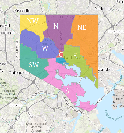
Source: Baltimore City Planning Department.

The results from the first query can also be visualized as shown below, by precinct:

# Nature of Homicides

Organize the data considering the nature of the homicide:

SELECT tags.type, count(*)
  FROM "row_number.3w4d-kckv"
GROUP BY tags.type
  ORDER BY count(*) DESC

Because of the ORDER BY count(*) DESC command, the data is displayed in descending order.

| tags.type                | count(*) |
|--------------------------|----------|
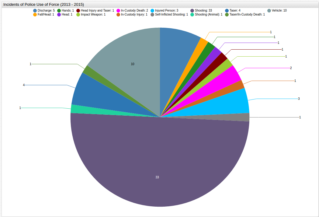
| Shooting                 | 33       |
| Vehicle                  | 10       |
| Discharge                | 5        |
| Taser                    | 4        |
| Head Injury              | 3        |
| Injured Person           | 3        |
| In Custody Death         | 2        |
| Fall/Head                | 1        |
| Taser / In Custody Death | 1        |
| Shooting (Animal)        | 1        |
| Self Inflicted Shooting  | 1        |
| Head Injury & Taser      | 1        |
| Impact Weapon            | 1        |
| In Custody Injury        | 1        |
| Hands                    | 1        |

Shown below is a visualization of three years' worth of incidents, sorted by the type of altercation:

# Date of Homicides

Organize the data considering the date of the homicide:

SELECT datetime, count(*)
  FROM "row_number.3w4d-kckv"
GROUP BY period(1 year)
  ORDER BY datetime

Notice here that the time aggregation interval is now set to 1 year because it is the variable being considered.

| datetime   | count(*) |
|------------|----------|
| 2013-01-01 | 12       |
| 2014-01-01 | 34       |
| 2015-01-01 | 22       |

Organize the data considering the month of the incident:

SELECT datetime, count(*)
  FROM "row_number.3w4d-kckv"
GROUP BY period(1 month, VALUE 0)
  ORDER BY datetime

| datetime   | count(*) |
|------------|----------|
| 2013-01-01 | 5        |
| 2013-02-01 | 0        |
| 2013-03-01 | 1        |
| 2013-04-01 | 2        |
| 2013-05-01 | 1        |
| 2013-06-01 | 0        |
| 2013-07-01 | 0        |
| 2013-08-01 | 1        |
| 2013-09-01 | 1        |
| 2013-10-01 | 1        |
| 2013-11-01 | 0        |
| 2013-12-01 | 0        |
| 2014-01-01 | 2        |
| 2014-02-01 | 4        |
| 2014-03-01 | 2        |
| 2014-04-01 | 2        |
| 2014-05-01 | 4        |
| 2014-06-01 | 3        |
| 2014-07-01 | 3        |
| 2014-08-01 | 7        |
| 2014-09-01 | 3        |
| 2014-10-01 | 0        |
| 2014-11-01 | 3        |
| 2014-12-01 | 1        |
| 2015-01-01 | 2        |
| 2015-02-01 | 3        |
| 2015-03-01 | 1        |
| 2015-04-01 | 4        |
| 2015-05-01 | 0        |
| 2015-06-01 | 2        |
| 2015-07-01 | 1        |
| 2015-08-01 | 0        |
| 2015-09-01 | 1        |
| 2015-10-01 | 2        |
| 2015-11-01 | 6        |

to maintain the chronology of the display, interpolation is used here to display those months without incident as well.

To view this table without interpolation see the Appendix

This data can be further visualized in ChartLab:

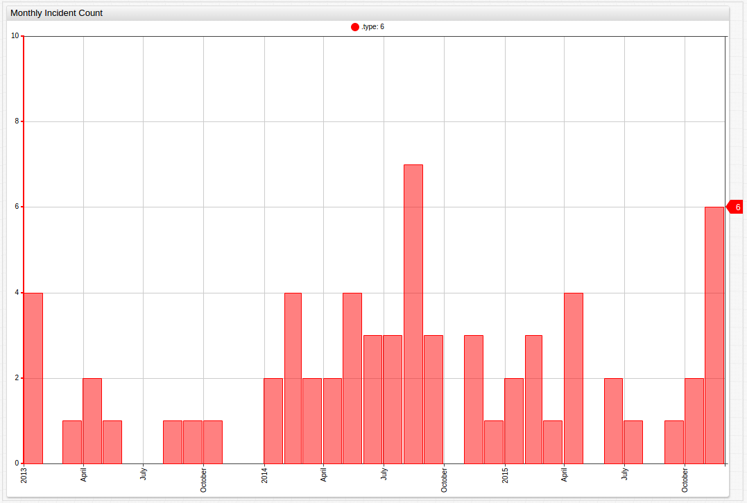
Because the nature of the visualization is such that the omission of empty months would distort the chronology of the data, interpolation is used once again.

Organize the data considering the week of the incident:

SELECT datetime, count(*)
  FROM "row_number.3w4d-kckv"
GROUP BY period(1 week)
  ORDER BY datetime

These results can also be visualized in ChartLab:

The day of the week of these incidents can also be considered using this query:

SELECT date_format(time, 'u'), count(*)
  FROM "row_number.3w4d-kckv"
GROUP BY date_format(time, 'u')

| date_format(time, 'u') | count(*) |
|------------------------|----------|
| 1                      | 11       |
| 2                      | 11       |
| 3                      | 9        |
| 4                      | 5        |
| 5                      | 9        |
| 6                      | 8        |
| 7                      | 15       |

When using the 'u' configuration in the DARE_FORMAT clause, the days of the week are displayed in order beginning with Monday, and represented with a number.

Using homicide data also provided by the City of Baltimore, the scale of police brutality can be shown alongside instances of homicide by civilians on other civilians. Does an increase in homicides result in an increase in police use of force? Do districts that see high levels of police use of force also see high levels of homicide? Is there a correlation at all?

Similar to the first data set, Socrata is used to compile the data in meaningful way and a Structured Query Language is used once again.

For a more detailed explanation of performing SQL Queries, see the Appendix below

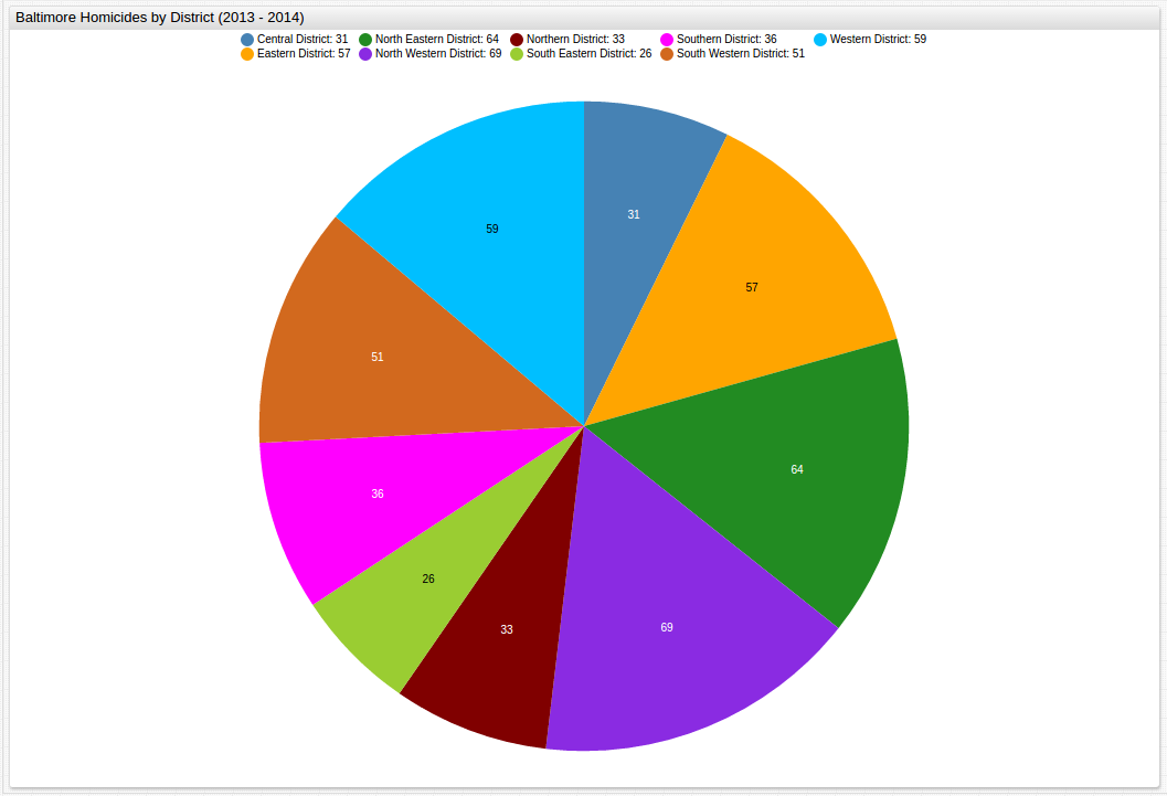
# District of Homicides

Organize the data considering the location of the incident:

SELECT tags.district, count(*)
  FROM "row_number.33zm-qy8h"
GROUP BY tags.district
  ORDER BY tags.district

| tags.district | count(*) |
|---------------|----------|
| CENTRAL       | 31       |
| EASTERN       | 57       |
| NORTHEASTERN  | 64       |
| NORTHERN      | 33       |
| NORTHWESTERN  | 69       |
| SOUTHEASTERN  | 26       |
| SOUTHERN      | 36       |
| SOUTHWESTERN  | 51       |
| WESTERN       | 59       |

A second visualization of the data shows nearly identical results to those seen above, the rates of homicides and incidents of police use of force follow a similar pattern:

Using a side-by-side comparison in ChartLab, the data can be viewed even more precisely, and the relationship between incidents resulting in the use of force by police, the local rate of homicide, and the location of the incident is underscored:

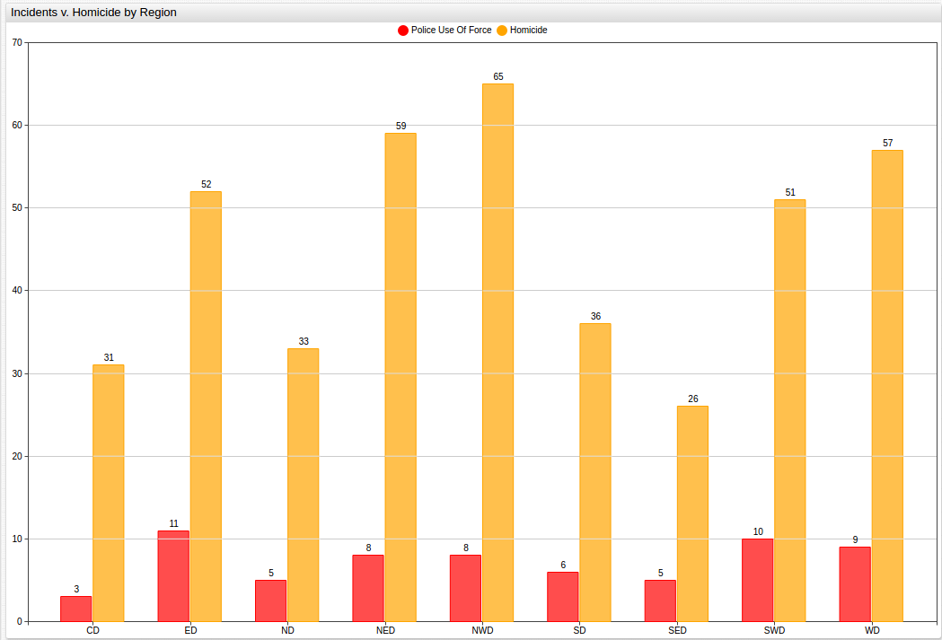
Although the recorded incidents of police use of force are not necessarily fatal, for the given time period eight of them resulted in the death of the victim, there is ostensibly a correlation between incidents of homicide and incidents of police use of force when the data is controlled for location. Areas with a higher frequency of homicides often see an increase in the number of events that the Baltimore Police use force to apprehend someone with whom they come in contact.

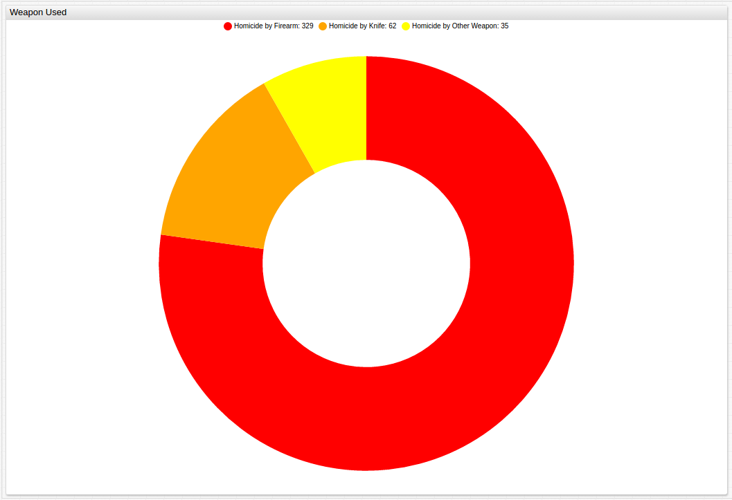
# Weapon of Homicides

The City of Baltimore includes figures that consider the weapon used in the commission of recorded homicides, queried in SQL Console:

SELECT tags.weapon, count(*)
  FROM "row_number.33zm-qy8h"
GROUP BY tags.weapon
  ORDER BY tags.weapon

Unsurprisingly, firearms are the primary tool of homicide for the observed period.

| tags.weapon | count(*) |
|-------------|----------|
| FIREARM     | 329      |
| KNIFE       | 62       |
| OTHER       | 35       |

These results can be shown graphically as well:

To organize the data considering the year of the incident:

SELECT datetime, count(*)
  FROM "row_number.33zm-qy8h"
GROUP BY period (1 year)
  ORDER BY datetime

| datetime   | count(*) |
|------------|----------|
| 2013-01-01 | 222      |
| 2014-01-01 | 204      |

Because of the way the data is stored, modifications need to be made to the way the collector reads the data for effective use, see the Action Items below for the assignment code needed.

Organize the data considering the month of the incident:

SELECT datetime, count(*)
  FROM "row_number.33zm-qy8h"
GROUP BY period (1 month)
  ORDER BY datetime

| datetime   | count(*) |
|------------|----------|
| 2013-01-01 | 14       |
| 2013-02-01 | 13       |
| 2013-03-01 | 18       |
| 2013-04-01 | 20       |
| 2013-05-01 | 20       |
| 2013-06-01 | 24       |
| 2013-07-01 | 18       |
| 2013-08-01 | 15       |
| 2013-09-01 | 23       |
| 2013-10-01 | 18       |
| 2013-11-01 | 20       |
| 2013-12-01 | 19       |
| 2014-01-01 | 24       |
| 2014-02-01 | 10       |
| 2014-03-01 | 7        |
| 2014-04-01 | 12       |
| 2014-05-01 | 22       |
| 2014-06-01 | 18       |
| 2014-07-01 | 21       |
| 2014-08-01 | 26       |
| 2014-09-01 | 18       |
| 2014-10-01 | 18       |
| 2014-11-01 | 13       |
| 2014-12-01 | 15       |

Using ChartLab, a side-by-side comparison of incidents of police use of force and homicides in the city of Baltimore can be done on a monthly basis:

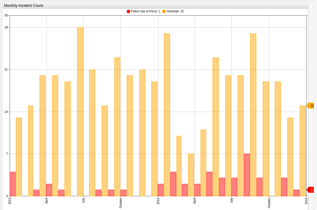
Here, the same correlation is less visible, with only one of the three spikes in homicides matched by a similar spike in police use of force.

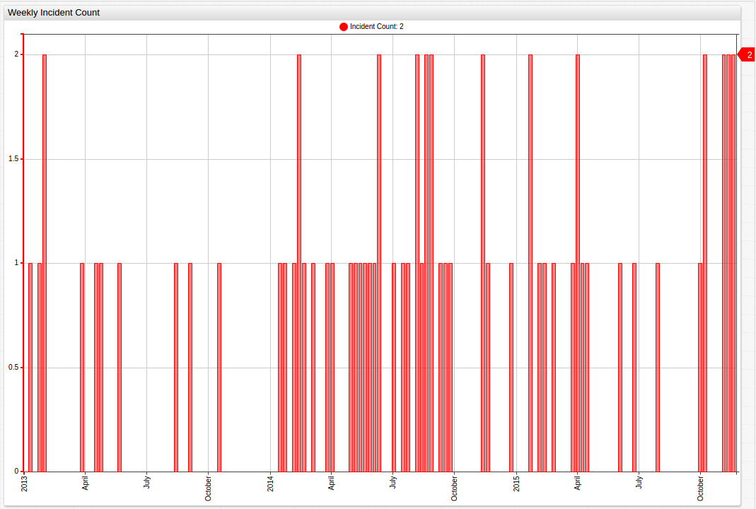
Likewise, a side-by-side comparison of incidents of police use of force and homicides in the city of Baltimore can be done on a weekly basis:

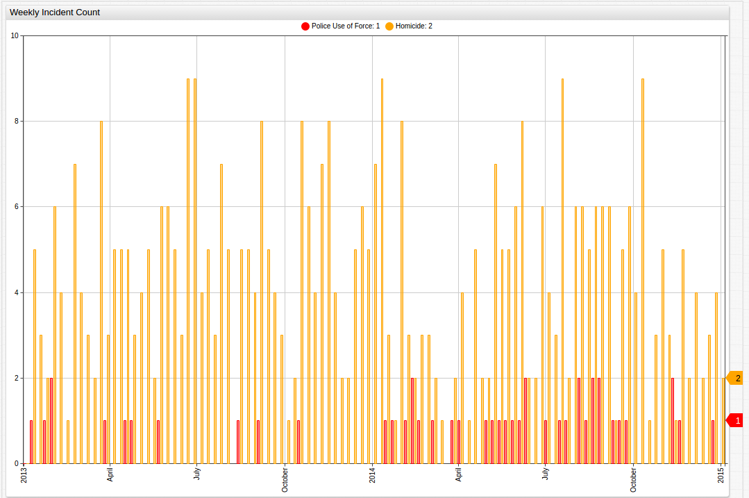
Here, the peaks in police use of force are further smoothed to indicate that the hypothetically resultant increase in police use of force occurs on a somewhat delayed basis after a spike in the number of homicides.

Notice that in ChartLab, the end-time setting must be modified to reflect the difference in observation periods between the two data sets.

Organize the data considering the day of the week:

SELECT date_format(time, 'u'), count(*)
  FROM "row_number.33zm-qy8h"
GROUP BY date_format(time, 'u')

| date_format(time, 'u') | count(*) |
|------------------------|----------|
| 1                      | 52       |
| 2                      | 70       |
| 3                      | 49       |
| 4                      | 58       |
| 5                      | 71       |
| 6                      | 64       |
| 7                      | 62       |

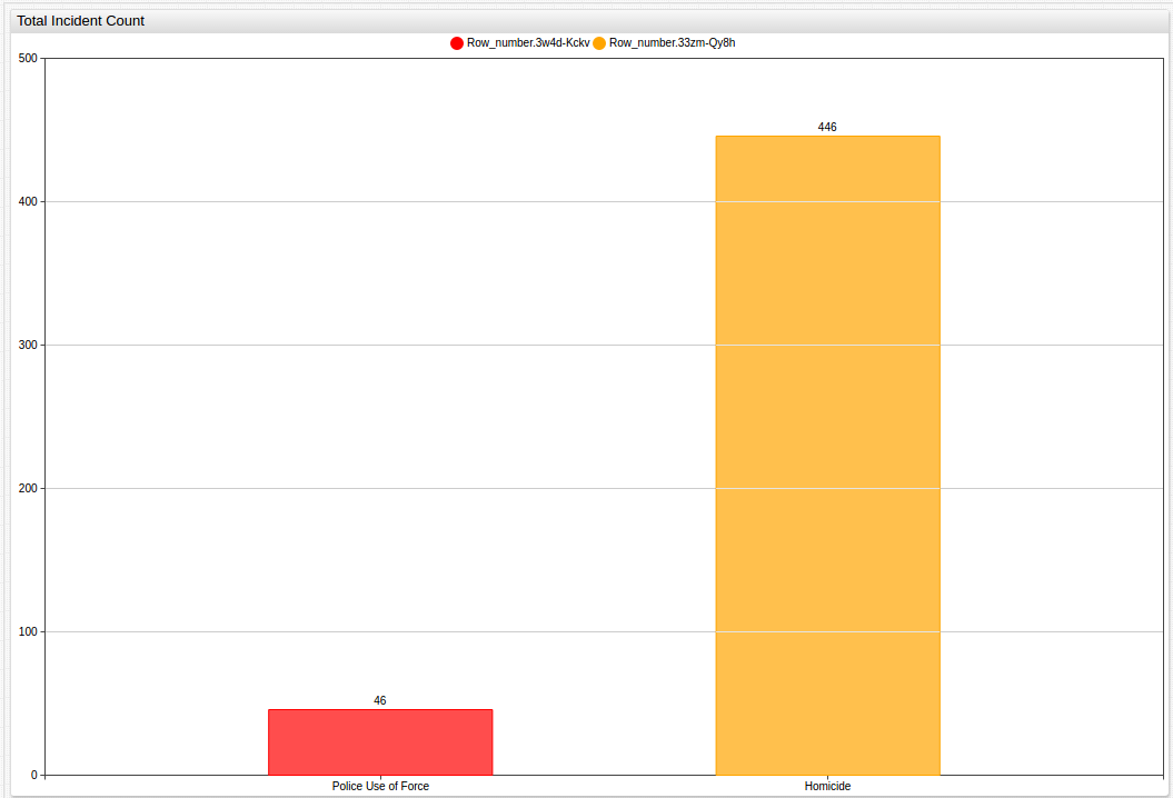
The above datasets can be combined to show the total number of incidents of police use of force and homicides over the span of the entire observed period.

# Analysis

The baseline average for number of homicides in a given Baltimore neighborhood was 47 (47.33) for the given time period. The average number of incidents of police use of force is 7 (7.22) during the same time period. If the null hypothesis is to be rejected and the alternative hypothesis considered to be at least possibly true, an above average amount of homicides in a given neighborhood should predict an above average number of incidents of police use of force.

Neighborhood	O1 (Homicide)	E1 (Homicide)	O2(Police)	E2 (Police)
Central	31	47	3	7
Eastern	57	47	11	7
Northeastern	64	47	8	7
North	33	47	5	7
Northwestern	69	47	8	7
Southeastern	26	47	5	7
Southern	36	47	6	7
Southwestern	51	47	10	7
Western	59	47	9	7

The trend is effectively predicted using the model described in Methodology.

Neighborhood	O1/E1	O2/E2
Central	0.6596	0.4286
Eastern	1.2128	1.5714
Northeastern	1.3617	1.1429
North	0.7021	0.7143
Northwestern	1.4681	1.1429
Southeastern	0.5532	0.7143
Southern	0.7660	0.8571
Southwestern	1.0851	1.4286
Western	1.2553	1.2857

The mean value of O1/E1 is 1.0426 and the standard deviation is 0.3398. The mean value of O2/E2 is 1.0317 and the standard deviation is 0.3765.

Neighborhood	(O1-E1)^2/E1	(O2-E2)^2/E2
Central	5.4460	2.2857
Eastern	1.7544	2.2857
Northeastern	4.5156	0.1429
North	4.1702	0.5714
Northwestern	9.3830	0.1429
Southeastern	9.3830	0.5714
Southern	2.5745	0.1429
Southwestern	0.3404	1.2857
Western	3.0638	0.5714

The p-value for the given series is 0.002, which is well within the acceptable range of significance, generally set around 0.05. Keep in mind, p-value is used to reject the null hypothesis but does not indicate the absolute validity of the alternative hypothesis.

After the death of Freddie Gray at the hands of the Baltimore Police Department in 2015, widespread protests broke out across the country with the epicenter of the demonstrations in the city of Baltimore itself. These demonstrations quickly led to violence, with drugstores looted, vehicles set on fire, and police officers and protesters alike injured in the ensuing melee. The city was ultimately placed under an official state of emergency by the Governor of Maryland and the State National Guard deployed to quash the unrest. The incident brought to light a range of issues with the way the American police force deals with the people they are sworn to protect and serve.

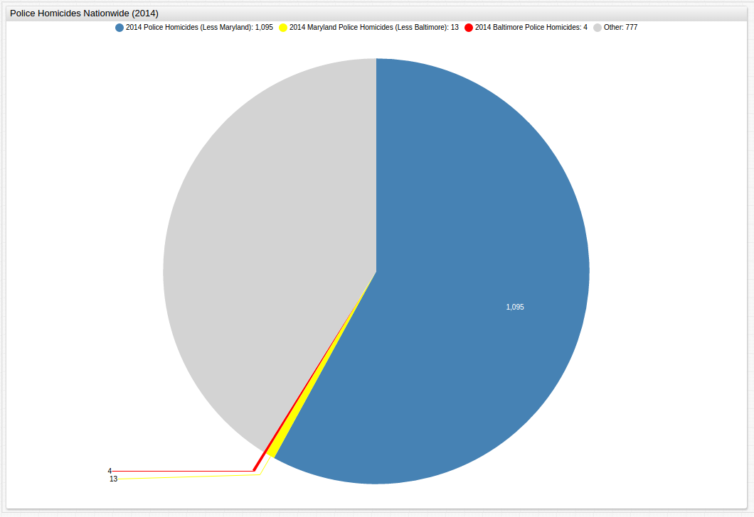
Across the entire United States, official data on people killed by the police is surprisingly difficult to find. Police agencies are not obligated to provide this data and as a result many of them do not. There are several citizen-run operations that collect data but the most reliable of these did not begin operation until May of 2013. Based on their figures, which cite news stories for each killing they claim, 777 Americans were killed in 2013 and 1,112 were killed in 2014 at the hands of the police. Fifteen of these victims were killed in the state of Maryland in 2013 and seventeen were killed in 2014. From these numbers, four victims were killed in Baltimore in 2013 and four more were killed in 2014. Officer-involved homicide made up 1.9% of total Baltimore homicides in 2013, and 1.8% of total Baltimore homicides in 2014.

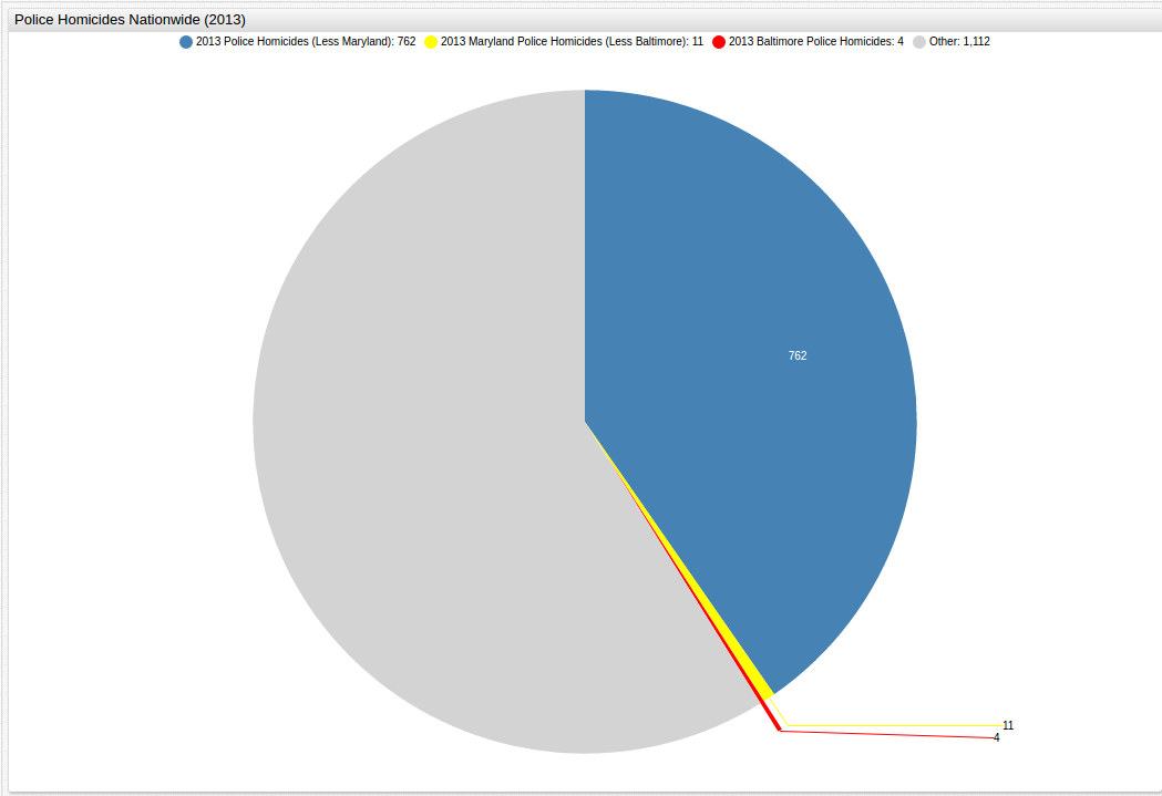
to display the total number of police homicides for the observed years, the [other] function can be used, only displaying data for the specified year, but still showing other data alongside for perspective.

See the Appendix below for more detailed instructions.

The protest actions centered around the claim that the death of Mr. Gray was yet another unneeded and careless casualty at the hands of a violent and overly-militarized police force, and official inability to explain the incident clearly only frustrated those who felt that the problem was far from resolved by their internal investigations. Countless stories have been published by various media outlets that have both defended and defamed law enforcement officers and their actions. Using these two datasets, it can be shown that while there is certainly a strong correlation between police precincts that have a high rate of homicide and the number of incidents that involve police use of force, the classic paradigm of the chicken and its egg come to mind. When trying to draw correlation on a short-term basis by comparing incidents of murder followed by incidents of police use of force, theoretically indicating that in precincts where a murder occurs, the following days are likely to see an incident of police violence the data shown above just cannot support the claim. Likewise the opposite claim, that precincts where the police use force to make an arrest are likely to have a homicide in the following days is equally unsupported by the data here. Perhaps the only true conclusion that can be drawn using such comparison methods is one that has been made since biblical times, reiterated again during the Civil Rights Movement by Martin Luther King, Jr: "Violence begets more violence." A total of six officers would be indicted and charged in a second-degree murder case that would ultimately see all six either acquitted, released on a mistrial, or free to go because the charges against them were dropped. Now, as the incident fades into memory, questions still remain about the ability of the citizenry to police the police, and thankfully, public data is available that allows them to do just that.

# Action Items

1. Download Docker.
2. Download the docker-compose.yml file to launch the ATSD container bundle.
3. Launch containers by specifying the built-in collector account credentials that are used by Axibase Collector to insert data into ATSD.

export C_USER=myuser; export C_PASSWORD=mypassword; docker-compose pull && docker-compose up -d

Note that both data sets have been collected under one Socrata job.

Contact Axibase with any questions.

# Appendix

# Using the expand Setting

to highlight specific data, as shown in the Nature of the Homicides section, use the expand setting under the [series] heading:

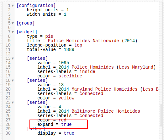
# Using the [other] Setting

to display a full series of data, but only show detailed information for a specified portion of that data, the [other] command needs to be included in the [series] cluster, and a value for total-value = x needs to be added under the [widget] cluster as shown below,

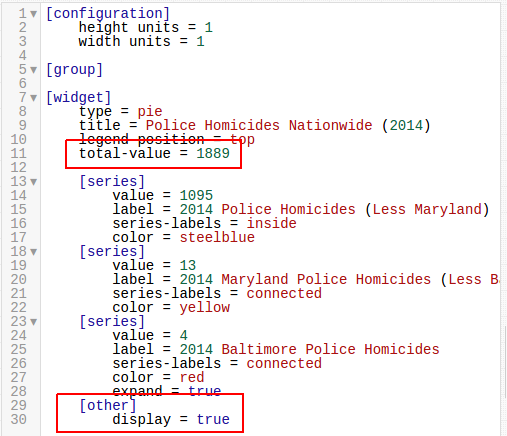
The default setting for the [other] command is false. If the display = true command is not entered, the visualization lacks total-value information.

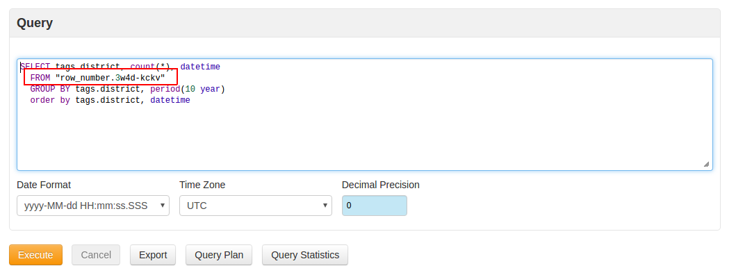
# Performing Queries in SQL Console

SELECT tags.$TAG_NAME$, count(*), datetime
  FROM "row_number.3w4d-kckv"
GROUP BY tags.$TAG_NAME$, PERIOD(1 MONTH)
  ORDER BY tags.$TAG_NAME$, datetime

Using this generic model, a series of queries can be performed in SQL Console.

The tags.$TAG_NAME$ corresponds to the metric the user is interested in querying.

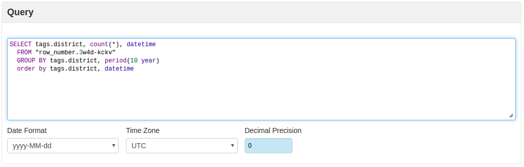
With the results displayed below, after the execute command is given. Erroneous data, or data lacking the target information is displayed as null.

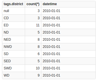
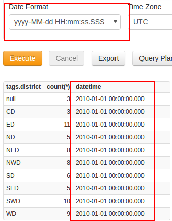
The datetime column can be modified to display day in any desirable format, in cases of data with more specific time specifications:

Changing between data sets only requires the modification of one line:

When controlling this data for time, because the data has been collected and stored as a time series, no additional tags commands are needed, but a slightly different syntax is used:

SELECT datetime, count(*)
  FROM "row_number.3w4d-kckv"
GROUP BY period(1 day)
  ORDER BY datetime

The period of observation can be modified on the third line using a myriad of time units.

# Monthly Police Incident Data Without Interpolation

SELECT datetime, count(*)
  FROM "row_number.3w4d-kckv"
GROUP BY period(1 month)
  ORDER BY datetime

Removing the VALUE 0 clause from the GROUP BY command renders the chart without interpolation.

| datetime   | count(*) |
|------------|----------|
| 2013-01-01 | 5        |
| 2013-03-01 | 1        |
| 2013-04-01 | 2        |
| 2013-05-01 | 1        |
| 2013-08-01 | 1        |
| 2013-09-01 | 1        |
| 2013-10-01 | 1        |
| 2014-01-01 | 2        |
| 2014-02-01 | 4        |
| 2014-03-01 | 2        |
| 2014-04-01 | 2        |
| 2014-05-01 | 4        |
| 2014-06-01 | 3        |
| 2014-07-01 | 3        |
| 2014-08-01 | 7        |
| 2014-09-01 | 3        |
| 2014-11-01 | 3        |
| 2014-12-01 | 1        |
| 2015-01-01 | 2        |
| 2015-02-01 | 3        |
| 2015-03-01 | 1        |
| 2015-04-01 | 4        |
| 2015-06-01 | 2        |
| 2015-07-01 | 1        |
| 2015-09-01 | 1        |
| 2015-10-01 | 2        |
| 2015-11-01 | 6        |

Contact Axibase with any questions.