Modeling Falling Birthrates in the Prairie State

Introduction
Long-considered to be a bellwether for trends in the rest of the country, the 21st state has grown from a tiny, sparsely-populated part of the Northwest Territory to the home of Chicago, the third-largest city in the country. Illinois holds the headquarters to some of the largest and most successful corporations in the United States including Boeing, Walgreens Boots Alliance, McDonald's, Sears Holdings, and United Continental. The University of Chicago has contributed countless innovations to the fields of business, economics, law, political science, and physics, among others, and is consistently ranked among the ten best universities in the country. Occasionally marred by political corruption, five state governors have been found guilty of misuse of power since the 1920's and a number of other state officials have also served time in prison as a result of their actions in office.
Home to some of America's favorite anti-heroes like Charlie Birger and Al Capone as well as icons like former presidents Abraham Lincoln and Barack Obama, it is not hard to understand why Illinois is considered as diverse and unique as the country itself.
Using data stored in Axibase Dataset Catalog released by Illinois Center for Health Statistics that covers two decades of live births in the state, from 1989 to 2009. This data has been kept through some of the formative events of the 20th and 21st centuries: the fall of the Berlin Wall, the World Trade Center terrorist attacks, the Pathfinder mission to Mars, the completion of the Burj Khalifa, and the emergence of the Internet to name a few.
Using the ATSD and the open source modelling software Fityk, the ICHS data can be visualized, modeled, and analyzed to extract valuable information from free public data.
Data
Analysis of these data has been divided into three sections, the first uses visualization to capture the information as a whole, the second queries the data in SQL Console, and the third uses curve fitting to anticipate future birth rates.
Visualizations
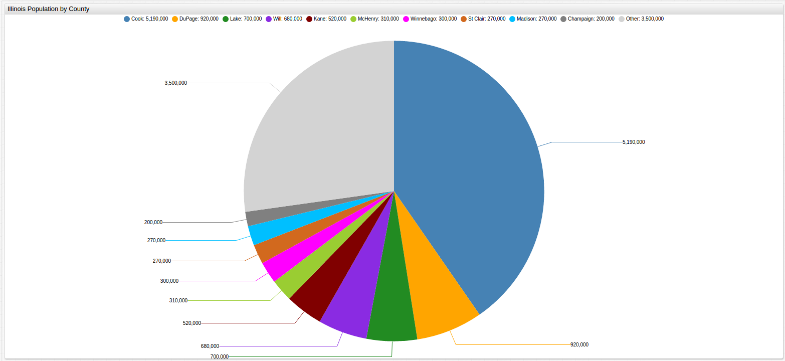
Illinois contains 102 counties, the top ten most populous of which are observed here. They are:
| Rank | County | County Seat | Population (Million) |
|---|---|---|---|
| 1 | Cook County | Chicago | 5.19 |
| 2 | DuPage County | Wheaton | 0.92 |
| 3 | Lake County | Waukegan | 0.70 |
| 4 | Will County | Joliet | 0.68 |
| 5 | Kane County | Geneva | 0.52 |
| 6 | McHenry County | Woodstock | 0.31 |
| 7 | Winnebago County | Rockford | 0.30 |
| 8 | St. Clair County | Belleville | 0.27 |
| 9 | Madison County | Edwardsville | 0.27 |
| 10 | Champaign County* | Urbana | 0.20 |
* Champaign County is the only top ten county by population not to appear as a top ten county by birthrate, consistently out-performed by the smaller Peoria County (Population: 0.19 million).
Open ChartLab to explore the number of live births in each of the counties listed above and navigate throughout the 20-year time period using the drop-down list at the top of the display.
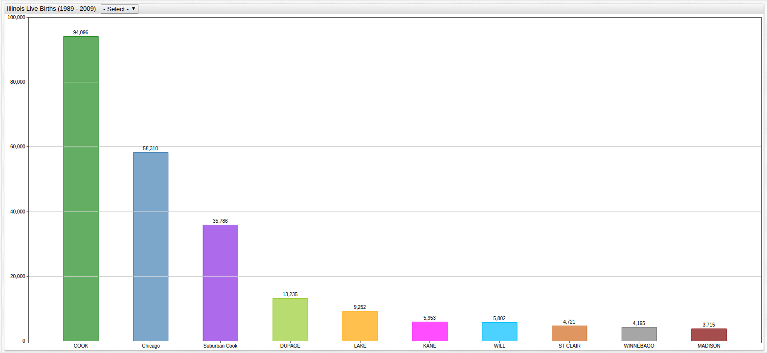

Learn more about creating a drop-down list in ChartLab in the Appendix below.
Use the ChartLab model below to compare the Top 10 counties' live births against the whole of Illinois' live births. Toggle between observed years using the drop-down list:
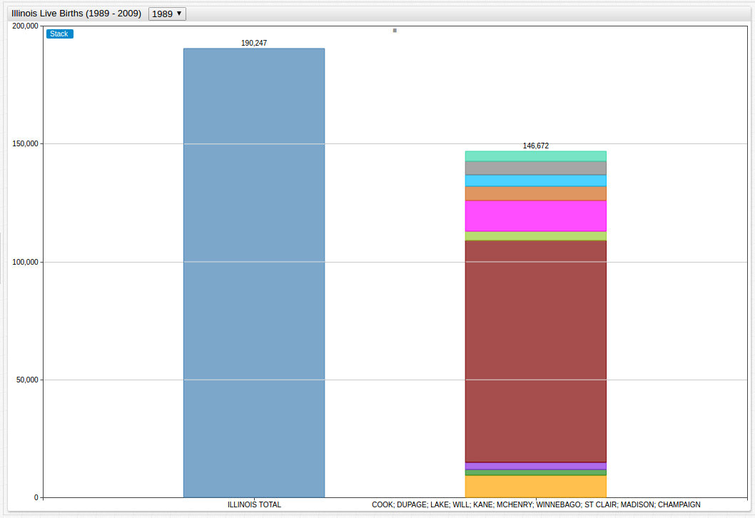
The ChartLab model below displays the same data, with those births not included in the top ten counties displayed in grey:
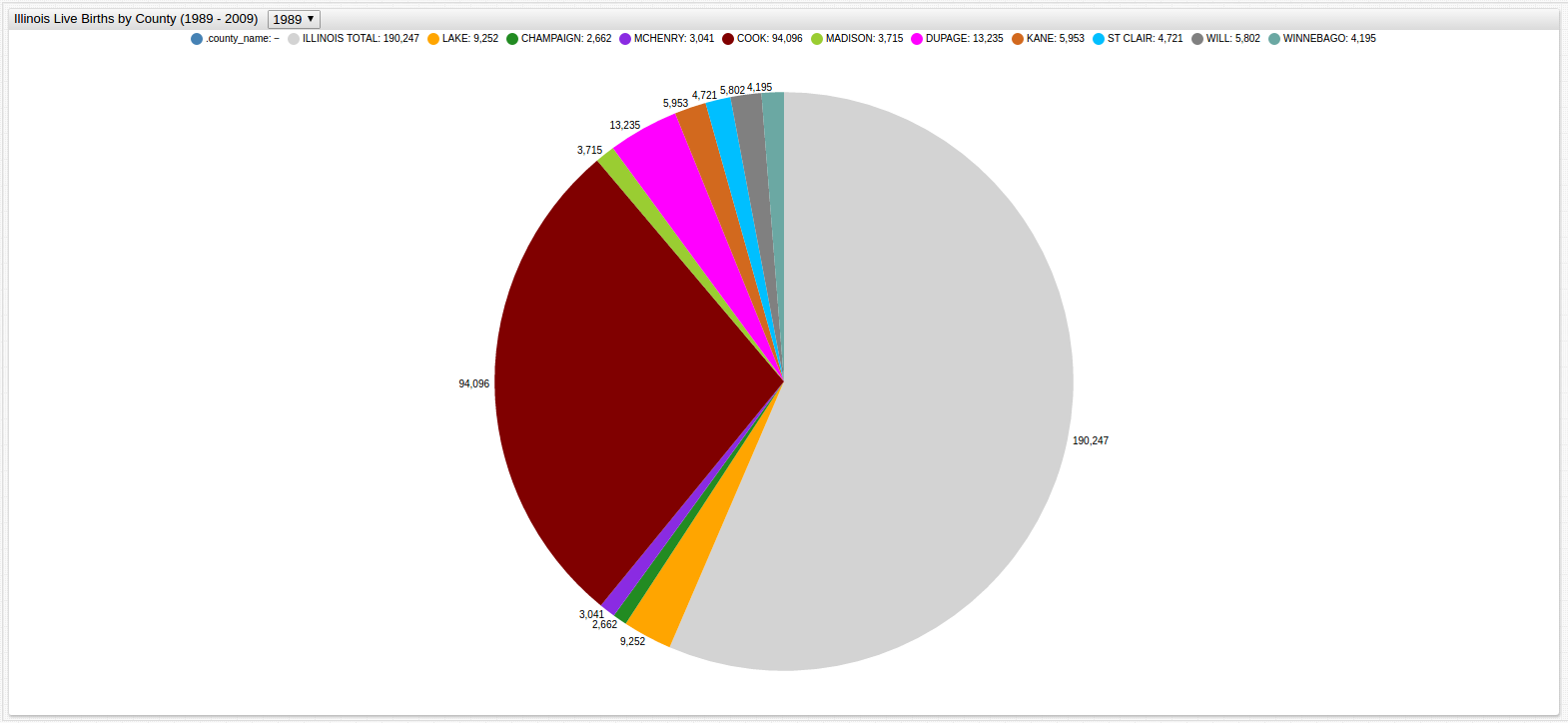
Removing the Illinois total numbers, and observing the live births by year from each of the ten largest counties:
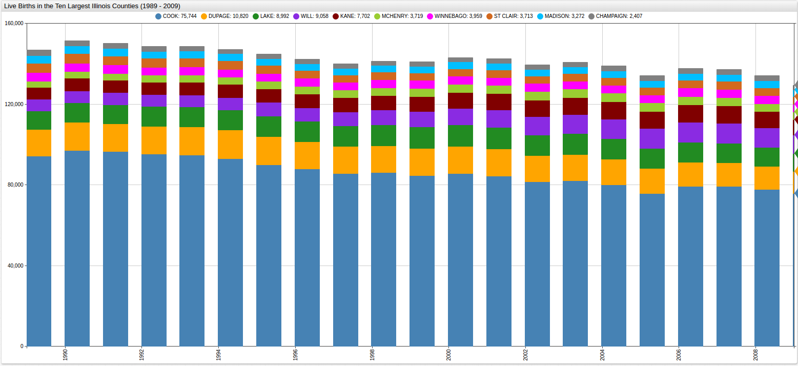
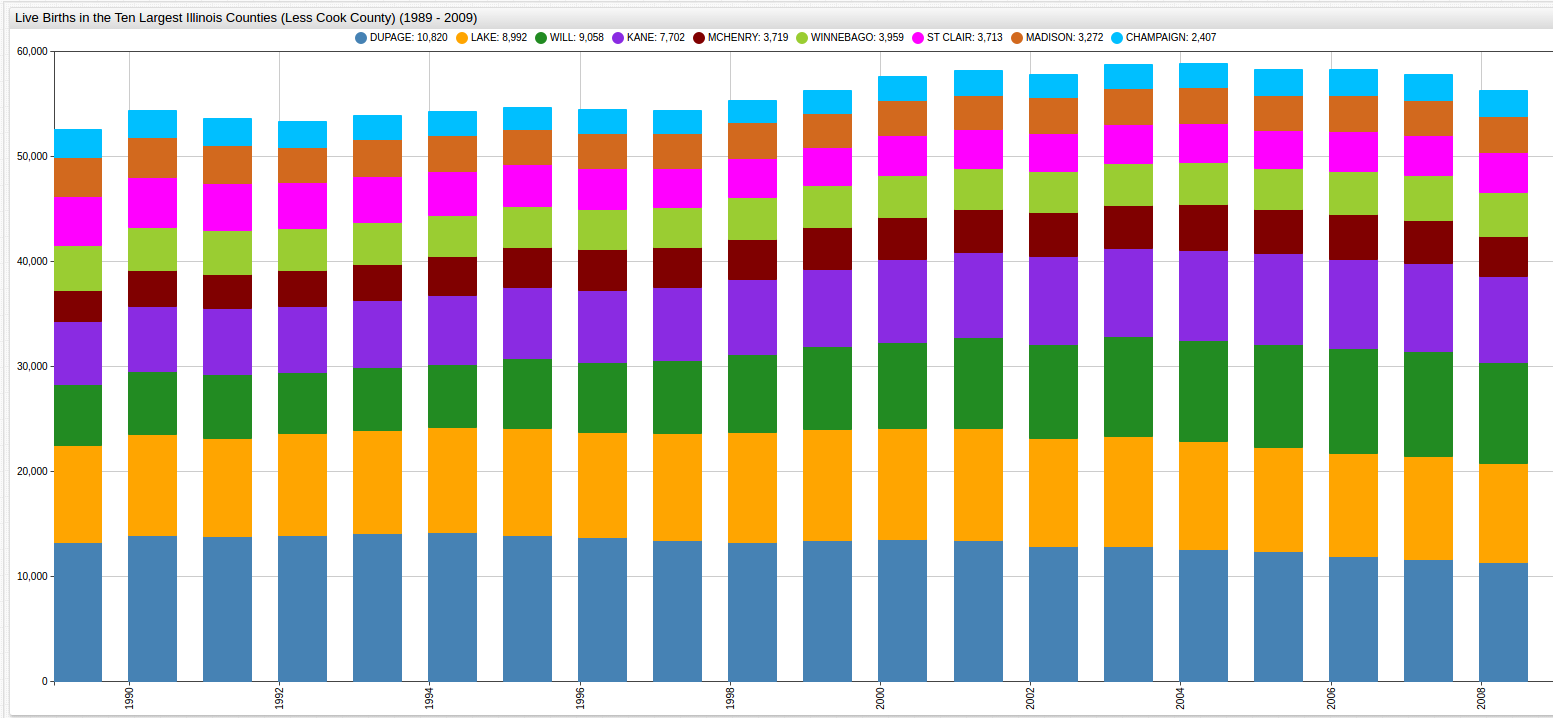
Now removing Cook County figures, as they represent the majority of Illinois live births:
Now looking at the whole of Illinois live birth rates, not just those from the most populous regions, their performance can be contrasted with the performance of the state as a whole:
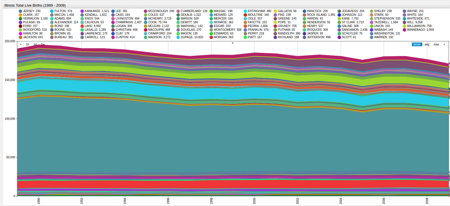
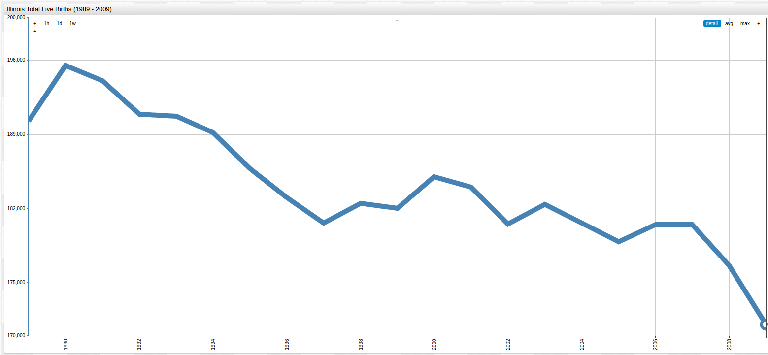
Illinois birthrates have been steadily declining for the past several decades.
A simplified version of the above figure shows only Illinois total live births, from 1989 to 2009:
SQL Queries
The data is difficult to work with because of the way it is stored. Typically, time information is
stored within a given metric, but in this case, each year is a metric in and of itself. This
type of storage can present a number of challenges for less detail-oriented software, but using the
ATSD and the supported JOIN clause,
working with, and analyzing even unideal data is well within the scope of possibility.
Birth numbers can be gathered in five-year steps:
1989
SELECT VALUE/1000 AS "Live Births (1000)", tags.county_name AS "County"
  FROM 1989 WHERE 'County' NOT IN ('Chicago', 'Suburban Cook')
GROUP BY tags.county_name, VALUE
  ORDER BY VALUE DESC, tags.county_name
LIMIT 11
| Live Births (1000) | County |
|---|---|
| 190 | ILLINOIS TOTAL |
| 94 | COOK |
| 13 | DUPAGE |
| 9 | LAKE |
| 6 | KANE |
| 6 | WILL |
| 5 | ST CLAIR |
| 4 | WINNEBAGO |
| 4 | MADISON |
| 3 | MCHENRY |
| 3 | PEORIA |
1994
SELECT VALUE/1000 AS "Live Births (1000)", tags.county_name AS "County"
  FROM 1994 WHERE 'County' NOT IN ('Chicago', 'Suburban Cook')
GROUP BY tags.county_name, VALUE
  ORDER BY VALUE DESC, tags.county_name
LIMIT 11
| Live Births (1000) | County |
|---|---|
| 189 | ILLINOIS TOTAL |
| 93 | COOK |
| 14 | DUPAGE |
| 10 | LAKE |
| 7 | KANE |
| 6 | WILL |
| 4 | ST CLAIR |
| 4 | WINNEBAGO |
| 4 | MCHENRY |
| 3 | MADISON |
| 3 | PEORIA |
1999
SELECT VALUE/1000 AS "Live Births (1000)", tags.county_name AS "County"
  FROM 1999 WHERE 'County' NOT IN ('Chicago', 'Suburban Cook')
GROUP BY tags.county_name, VALUE
  ORDER BY VALUE DESC, tags.county_name
LIMIT 11
| Live Births (1000) | County |
|---|---|
| 182 | ILLINOIS TOTAL |
| 85 | COOK |
| 13 | DUPAGE |
| 11 | LAKE |
| 8 | WILL |
| 7 | KANE |
| 4 | MCHENRY |
| 4 | WINNEBAGO |
| 4 | ST CLAIR |
| 3 | MADISON |
| 3 | PEORIA |
2004
SELECT VALUE/1000 AS "Live Births (1000)", tags.county_name AS "County"
  FROM 2004 WHERE 'County' NOT IN ('Chicago', 'Suburban Cook')
GROUP BY tags.county_name, VALUE
  ORDER BY VALUE DESC, tags.county_name
LIMIT 11
| Live Births (1000) | County |
|---|---|
| 181 | ILLINOIS TOTAL |
| 80 | COOK |
| 13 | DUPAGE |
| 10 | LAKE |
| 10 | WILL |
| 9 | KANE |
| 4 | MCHENRY |
| 4 | WINNEBAGO |
| 4 | ST CLAIR |
| 3 | MADISON |
| 3 | PEORIA |
2009
SELECT VALUE/1000 AS "Live Births (1000)", tags.county_name AS "County"
  FROM 2009 WHERE 'County' NOT IN ('Chicago', 'Suburban Cook')
GROUP BY tags.county_name, VALUE
  ORDER BY VALUE DESC, tags.county_name
LIMIT 11
| Live Births (1000) | County |
|---|---|
| 171 | ILLINOIS TOTAL |
| 76 | COOK |
| 11 | DUPAGE |
| 9 | WILL |
| 9 | LAKE |
| 8 | KANE |
| 4 | WINNEBAGO |
| 4 | MCHENRY |
| 4 | ST CLAIR |
| 3 | MADISON |
| 3 | PEORIA |
Likewise, county totals can be gathered using the same five-year steps, but evaluating for the entire observed time and not one-year segments:
1989 - 1993
SELECT (t1.VALUE + t2.VALUE + t3.VALUE + t4.VALUE + t5.VALUE)/1000 AS "Live Births (1000)", t1.tags.county_name AS "County"
  FROM 1989 t1 JOIN 1990 t2 JOIN 1991 t3 JOIN 1992 t4 JOIN 1993 t5
WHERE t1.tags.county_name = t2.tags.county_name AND t1.tags.county_name NOT IN ('Chicago','Suburban Cook')
  GROUP BY t1.tags.county_name, t1.VALUE, t2.VALUE, t3.VALUE, t4.VALUE, t5.VALUE
ORDER BY t1.VALUE DESC, t1.tags.county_name
  LIMIT 11
| Live Births (1000) | County |
|---|---|
| 961 | ILLINOIS TOTAL |
| 477 | COOK |
| 69 | DUPAGE |
| 48 | LAKE |
| 31 | KANE |
| 30 | WILL |
| 23 | ST CLAIR |
| 21 | WINNEBAGO |
| 18 | MADISON |
| 16 | MCHENRY |
| 14 | PEORIA |
1994 - 1998
SELECT (t1.VALUE + t2.VALUE + t3.VALUE + t4.VALUE + t5.VALUE)/1000 AS "Live Births (1000)", t1.tags.county_name AS "County"
  FROM 1994 t1 JOIN 1995 t2 JOIN 1996 t3 JOIN 1997 t4 JOIN 1998 t5
WHERE t1.tags.county_name = t2.tags.county_name AND t1.tags.county_name NOT IN ('Chicago','Suburban Cook')
  GROUP BY t1.tags.county_name, t1.VALUE, t2.VALUE, t3.VALUE, t4.VALUE, t5.VALUE
ORDER BY t1.VALUE DESC, t1.tags.county_name
  LIMIT 11
| Live Births (1000) | County |
|---|---|
| 921 | ILLINOIS TOTAL |
| 442 | COOK |
| 69 | DUPAGE |
| 51 | LAKE |
| 34 | KANE |
| 34 | WILL |
| 20 | ST CLAIR |
| 19 | WINNEBAGO |
| 19 | MCHENRY |
| 17 | MADISON |
| 13 | PEORIA |
1999 - 2003
SELECT (t1.VALUE + t2.VALUE + t3.VALUE + t4.VALUE + t5.VALUE)/1000 AS "Live Births (1000)", t1.tags.county_name AS "County"
  FROM 1999 t1 JOIN 2000 t2 JOIN 2001 t3 JOIN 2002 t4 JOIN 2003 t5
WHERE t1.tags.county_name = t2.tags.county_name AND t1.tags.county_name NOT IN ('Chicago','Suburban Cook')
  GROUP BY t1.tags.county_name, t1.VALUE, t2.VALUE, t3.VALUE, t4.VALUE, t5.VALUE
ORDER BY t1.VALUE DESC, t1.tags.county_name
  LIMIT 11
| Live Births (1000) | County |
|---|---|
| 914 | ILLINOIS TOTAL |
| 418 | COOK |
| 66 | DUPAGE |
| 53 | LAKE |
| 43 | WILL |
| 40 | KANE |
| 21 | MCHENRY |
| 20 | WINNEBAGO |
| 18 | ST CLAIR |
| 17 | MADISON |
| 13 | PEORIA |
2004 - 2008
SELECT (t1.VALUE + t2.VALUE + t3.VALUE + t4.VALUE + t5.VALUE)/1000 AS "Live Births (1000)", t1.tags.county_name AS "County"
  FROM 2004 t1 JOIN 2005 t2 JOIN 2006 t3 JOIN 2007 t4 JOIN 2008 t5
WHERE t1.tags.county_name = t2.tags.county_name AND t1.tags.county_name NOT IN ('Chicago','Suburban Cook')
  GROUP BY t1.tags.county_name, t1.VALUE, t2.VALUE, t3.VALUE, t4.VALUE, t5.VALUE
ORDER BY t1.VALUE DESC, t1.tags.county_name
  LIMIT 11
| Live Births (1000) | County |
|---|---|
| 897 | ILLINOIS TOTAL |
| 392 | COOK |
| 60 | DUPAGE |
| 49 | LAKE |
| 49 | WILL |
| 42 | KANE |
| 21 | MCHENRY |
| 20 | WINNEBAGO |
| 19 | ST CLAIR |
| 17 | MADISON |
| 13 | PEORIA |
Information can also be collected on a specific county, for the entire period:
Cook County Live Births (1989 - 2009)
SELECT DATE_FORMAT(TIME, 'yyyy') AS "Year", tags.county_name AS "County", VALUE/100000 AS "Live Births (100000)"
  FROM "year.9e74-xdvk.value"
WHERE 'County' = 'COOK'
  GROUP BY 'County', VALUE, 'Year'
ORDER BY 'Year'
| Year | County | Live Births (100000) |
|---|---|---|
| 1989 | COOK | 0.94 |
| 1990 | COOK | 0.97 |
| 1991 | COOK | 0.96 |
| 1992 | COOK | 0.95 |
| 1993 | COOK | 0.95 |
| 1994 | COOK | 0.93 |
| 1995 | COOK | 0.90 |
| 1996 | COOK | 0.88 |
| 1997 | COOK | 0.86 |
| 1998 | COOK | 0.86 |
| 1999 | COOK | 0.85 |
| 2000 | COOK | 0.86 |
| 2001 | COOK | 0.84 |
| 2002 | COOK | 0.82 |
| 2003 | COOK | 0.82 |
| 2004 | COOK | 0.80 |
| 2005 | COOK | 0.76 |
| 2006 | COOK | 0.79 |
| 2007 | COOK | 0.79 |
| 2008 | COOK | 0.78 |
| 2009 | COOK | 0.76 |
Curve Fitting
Data points can also be collected using an SQL query.
Illinois Total Live Births:
SELECT DATE_FORMAT(TIME, 'yyyy') AS "Year", tags.county_name AS "County", VALUE/1000 AS "Live Births (1000)"
  FROM "year.9e74-xdvk.value"
WHERE 'County' = 'ILLINOIS TOTAL'
  GROUP BY 'County', VALUE, 'Year'
ORDER BY 'Year'
| Year | County | Live Births (1000) |
|---|---|---|
| 1989 | ILLINOIS TOTAL | 190 |
| 1990 | ILLINOIS TOTAL | 195 |
| 1991 | ILLINOIS TOTAL | 194 |
| 1992 | ILLINOIS TOTAL | 191 |
| 1993 | ILLINOIS TOTAL | 191 |
| 1994 | ILLINOIS TOTAL | 189 |
| 1995 | ILLINOIS TOTAL | 186 |
| 1996 | ILLINOIS TOTAL | 183 |
| 1997 | ILLINOIS TOTAL | 181 |
| 1998 | ILLINOIS TOTAL | 183 |
| 1999 | ILLINOIS TOTAL | 182 |
| 2000 | ILLINOIS TOTAL | 185 |
| 2001 | ILLINOIS TOTAL | 184 |
| 2002 | ILLINOIS TOTAL | 181 |
| 2003 | ILLINOIS TOTAL | 182 |
| 2004 | ILLINOIS TOTAL | 181 |
| 2005 | ILLINOIS TOTAL | 179 |
| 2006 | ILLINOIS TOTAL | 181 |
| 2007 | ILLINOIS TOTAL | 181 |
| 2008 | ILLINOIS TOTAL | 177 |
| 2009 | ILLINOIS TOTAL | 171 |
The dataset used for modeling is as follows:
| Year | X | Y |
|---|---|---|
| 1989 | 1 | 190 |
| 1990 | 2 | 195 |
| 1991 | 3 | 194 |
| 1992 | 4 | 191 |
| 1993 | 5 | 191 |
| 1994 | 6 | 189 |
| 1995 | 7 | 186 |
| 1996 | 8 | 183 |
| 1997 | 9 | 181 |
| 1998 | 10 | 183 |
| 1999 | 11 | 182 |
| 2000 | 12 | 185 |
| 2001 | 13 | 184 |
| 2002 | 14 | 181 |
| 2003 | 15 | 182 |
| 2004 | 16 | 181 |
| 2005 | 17 | 179 |
| 2006 | 18 | 181 |
| 2007 | 19 | 181 |
| 2008 | 20 | 177 |
| 2009 | 21 | 171 |
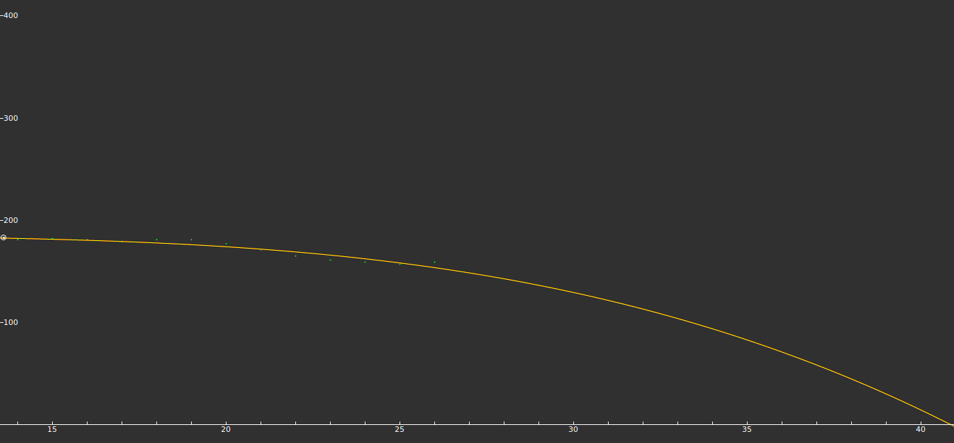
Using Fityk to create a best-fit model for this data:
Model One

The associated formula is shown below:
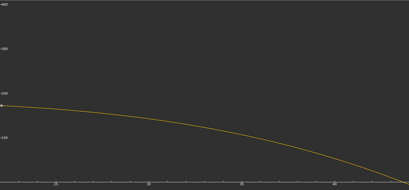
F(x) = 197 + -2.59*x + 0.179*x^2 + -0.00511*x^3
Moving the window to the right estimates the total live births for years not included in the table above:
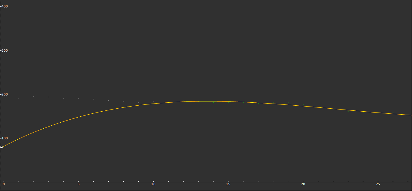
Excluding the final data point from the series, which deviated significantly, creates a less extreme model:
Model Two

The formula is shown here:
F(x) = 196 + -1.7*x + 0.0587*x^2 + -0.000794*x^3
And the same forward-shift of the viewing window:

To test the accuracy of each model, live birth figures from years not included in the data set but available from the Illinois Department of Public Health can be used, and WolframAlpha can manage the computations.
| Year | Live Births (Estimated) Model 1, Model 2 (Hundred Thousand) | Live Births (Actual) (Hundred Thousand) | % Error Model 1, Model 2 |
|---|---|---|---|
| 2010* | 172, 179 | 165 | 4.06%, 7.82% |
| 2011 | 169, 178 | 161 | 4.96%, 10.56% |
| 2012 | 167, 178 | 159 | 5.03%, 11.95% |
| 2013 | 164, 178 | 157 | 4.46%, 13.37% |
| 2014 | 160, 178 | 159 | 6.29%, 11.95% |
* Indicates a year in which the US Census is performed.
Model 1 more accurately predicts the results of recent live birth numbers, and the variance is reasonable, 0.7085. Model 2 less accurately predicts the results of recent live birth numbers and its variance is quite high, 4.4109. These numbers show the stability of the model over the course of a given period of time.
Despite its stability for the given data and relative accuracy in predicting birthrates outside of the training data, Model 1 begins to lose effectiveness about fifteen years outside of the originally observed period, underlining the importance of constantly updating and maintaining such models with new information.
When updated to include the latest figures, the model looks like this:
Model Three

The updated formula is shown here:
F(x) = 197 + -2.53*x + 0.189*x^2 + -0.006*x^3
The forward-shift is shown below:
Intuitively, this model appears flawed as it shows Illinois live births dropping to zero around the year 2038, but some of the older data can now be excluded, to reflect the trends of the last decade while excluding data that is two decades old and reflects the trends of a society that has experienced a wide array of dramatic changes:
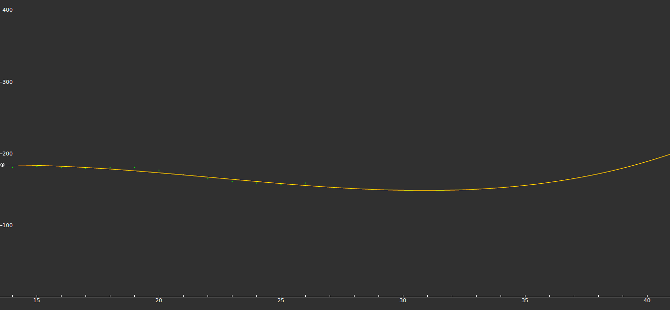
Model Four
The newly updated formula is shown here:
F(x) = 81.9 + 17.6*x + -0.929*x^2 + 0.0139*x^3
The forward-shift is shown below:
Considering population dynamics, such as human factors like economic opportunity, is also paramount when attempting to design models for a longer span of time, or for non-stationary populations.
Using model 4 to predict United States Census numbers for the next two Censuses is shown below:
| Census Year | Model 4 Prediction (Hundred Thousand Live Births) |
|---|---|
| 2020 | 149 |
| 2030 | 212 |
The instability that afflicted Model 1 too far outside the training data, appears to be at work here as well.
Conclusions
The falling Illinois birthrates have been noted by policy groups and investment firms that have expressed concern for the future of the Land of Lincoln. Some have noted the continued inability of Illinois residents to reproduce at replacement rates and pointed to formerly decadent American cities like Detroit as the likely outcome of the continuation of such trends, while others including the Center for Disease Control (CDC) have released predictions that claim that by the time of the 2020 Census, birthrates will have stabilized or even seen a surge similar to the one in the early 90's. The fourth model produced here predicted similar growth as well, showing a local minima during the year 2019 followed by growth in the number of live births the following year.
The only true certainty is that any such modeling should be taken with a grain of salt and interpreted with the understanding that such predictions are based on the continuation of current trends which can change quite quickly and sometimes unpredictably.
Appendix
Creating a Drop-Down List
For a complete walkthrough, refer to Drop-Down Lists.
Using the below chart as an example:
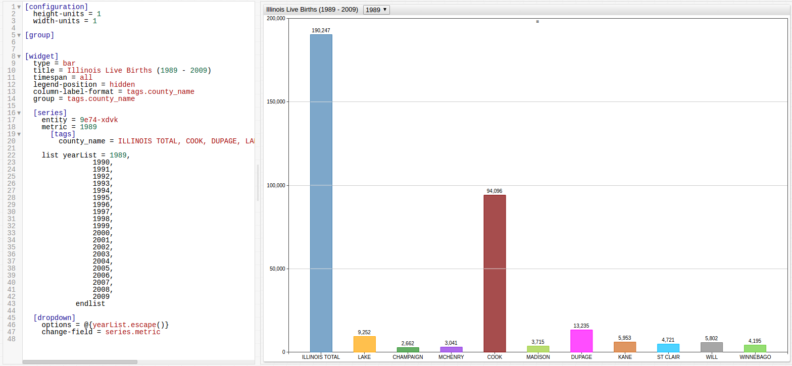
And looking at lines 22 - 48 in the Editor:
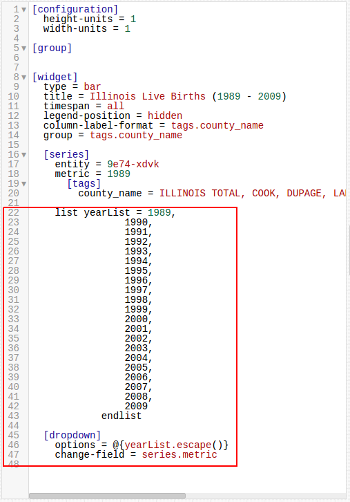
The LIST Setting is used to declare a specific list, in this case, the various
years of included in the data and the [dropdown]
heading is used to declare the functionality of the menu itself.
Action Items
- Download Docker.
- Download the
docker-compose.ymlfile to launch the ATSD container bundle. - Launch containers by specifying the built-in collector account credentials used by Axibase Collector to insert data into ATSD.
export C_USER=username; export C_PASSWORD=password; docker-compose pull && docker-compose up -d
Contact Axibase with any questions.