# Real-time Analysis of the Oroville Dam Disaster

In February 2017, reservoir levels for the tallest dam in the United States, located near Oroville, California, were beginning to reach capacity from high rainfall totals. Officials decided to begin using the primary dam spillway, which quickly began to deteriorate, and by February 10th, a hole 300 feet wide, 500 feet long, and 45 feet deep had appeared in the spillway. On February 11th, officials decided to begin using an auxiliary, spillway composed of earthen materials. The emergency spillway quickly began to erode as well. On February 12th, due to the "hazardous situation" surrounding the dam, more than 200,000 people from downstream communities were ordered to evacuate the area. In the early morning hours of February 13th, the reservoir water levels returned below the threshold capacity of the dam.

While the situation has calmed somewhat in the last several days, the crisis is by no means over. Rain has been forecast for the next several days. With a water surface area of 15,810 acres, the difference of mere inches of rain can make the difference between crisis averted and complete disaster for the Oroville dam.

This article analyzes a dataset from the California Department of Water Resources (CDWR) looking at the several vital statistics for the Oroville dam. This article provides real-time analysis with ChartLab graphs (updated hourly and automatically with data taken from the CDWR website), which show the current situation at the dam. Additionally, this article illustrates how publicly available data from CDWR can be easily loaded into the non-relational Axibase Time Series Database for interactive analysis with graphical representation of open data published by government organizations.

# Oroville Dam Dataset

Begin by gathering current data for the Oroville dam from cdec.water.ca.gov. This dataset can be found on the CDEC website.

Data is collected hourly for the Oroville dam for the following metrics:

• Reservoir Elevation (feet)
• Reservoir Storage (acre-foot)
• Dam Outflow (cubic feet/second)
• Dam Inflow (cubic feet/second)
• Spillway Outflow (cubic feet/second)
• Rain (inches)

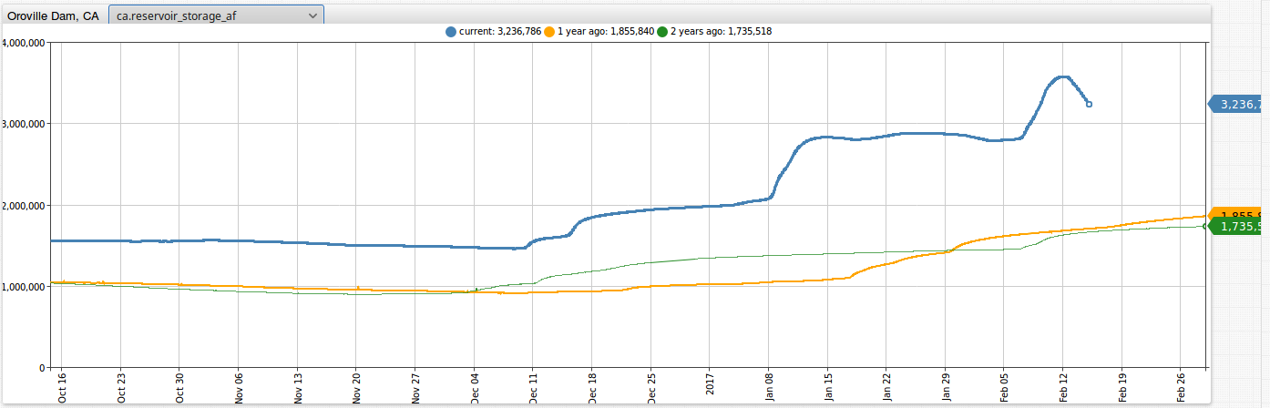
Below is an image showing these CDWR metrics in ATSD. You can toggle between the different metrics by clicking on the drop-down list.

You can explore the basic CDWR portal (loaded into ATSD) by clicking the button below:

You do not need to install ATSD to look the real-time Oroville dam analysis in this article.

You can, however, load the dataset into your ATSD instance by following the steps provided at the end of the article.

# The Current Situation - Real-time Analysis

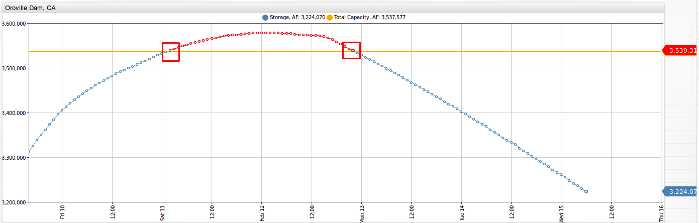
Below is a screenshot showing the change in storage capacity of the dam from Friday February 10th, 2017, to the morning of February 15th, 2017 (the time of publication). The threshold capacity is 3,537,577 AF, as marked by the orange line in the image. As a note, you can scroll over horizontally and up or down vertically by left-clicking and dragging in the direction you would like to shift. The approximate time that the dam exceeded the threshold capacity is between 2:00 and 3:00 am U.S. pacific time (PT) on February 11th. 3,539,160 AF is recorded at 2:00 am on February 11th, and the storage level returned to below the threshold limit between 11:00 pm on February 12th and 12:00 am (PT) on February 13th with 3,533,936 AF recorded at midnight (both times marked below). Additionally, the dam hit its peak overflow of 3,578,686 AF on Sunday February 12th at 3:00 am.

You can explore this portal by clicking the button below:

# Reservoir Storage Levels

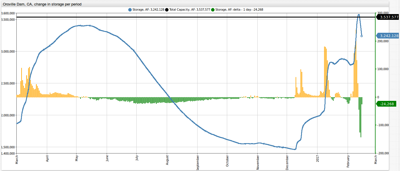
Below is an image showing the change in reservoir storage going back to March 2016 at the Oroville dam. The blue line represents the hourly, absolute value of the reservoir storage (in acre-feet), with values shown on the left hand side of the graph. Change in the dam storage is represented by the yellow and green columns: yellow represents an increase in the reservoir storage, while green represents a decrease (both in acre-feet per day). These delta values are displayed on the right hand side of the graph.

Zooming into the last couple of months, notice how storage levels are changing at the time of the dam overflow.

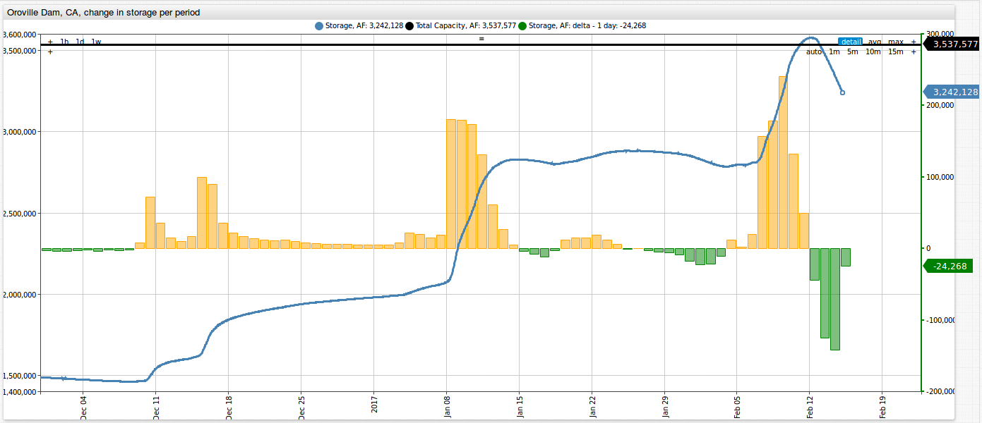
Reservoir levels experienced their first significant uptick on December 10th, 2016, with an increase of 34,571 AF added to the reservoir storage. Over the next several weeks, the dam experienced an increase in storage (with the exception of a handful of days). By toggling over each of the individual columns, notice the change in the storage for February 9th (237,689 AF), 10th (39,522 AF), and 11th (53,896 AF), which is when the dam was overtopped.

You can explore this portal by clicking on the button below:

# Reservoir Inflow, Outflows, and Precipitation

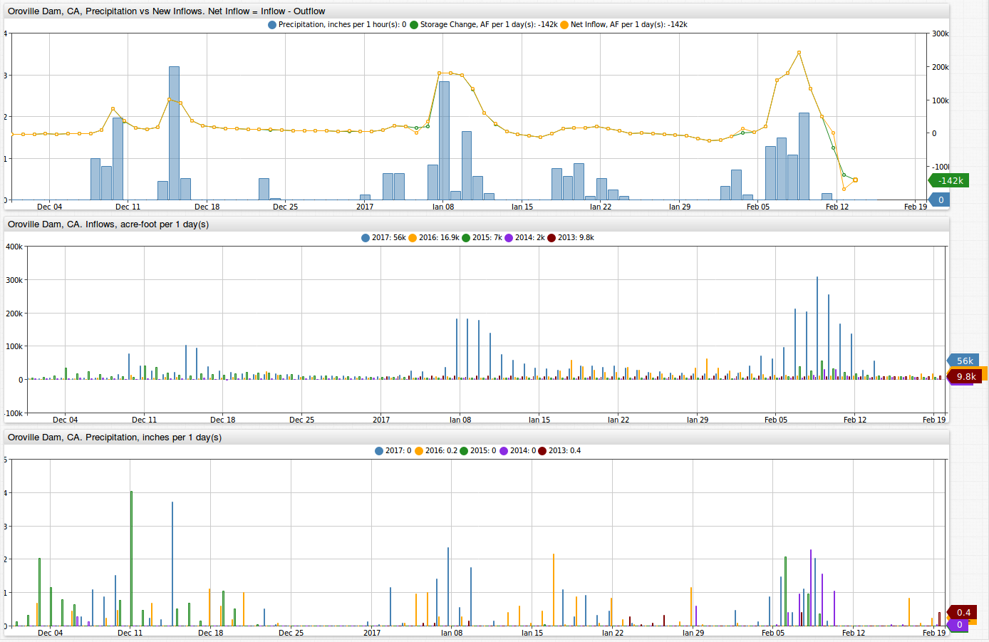
Below are three outputs for the Oroville dam:

• Precipitation vs new inflows, where net inflow is the difference between reservoir inflow and outflow. With this graph notice the relationship between precipitation totals and the net inflows/storage of the dam.
• Inflows (measured in acre-foot per day) for 2017, 2016, 2015, 2014, and 2013. From this visualization, it is clear that inflows for 2017 have been far greater than any of the recent previous years.
• Precipitation per day (inches) for 2017, 2016, 2015, 2014, and 2013. While inflows for 2017 are quite a bit greater than previous years totals precipitation totals in 2017 are not too far ahead of previous years.

You can explore this portal by clicking on the button below:

# The Next Several Days

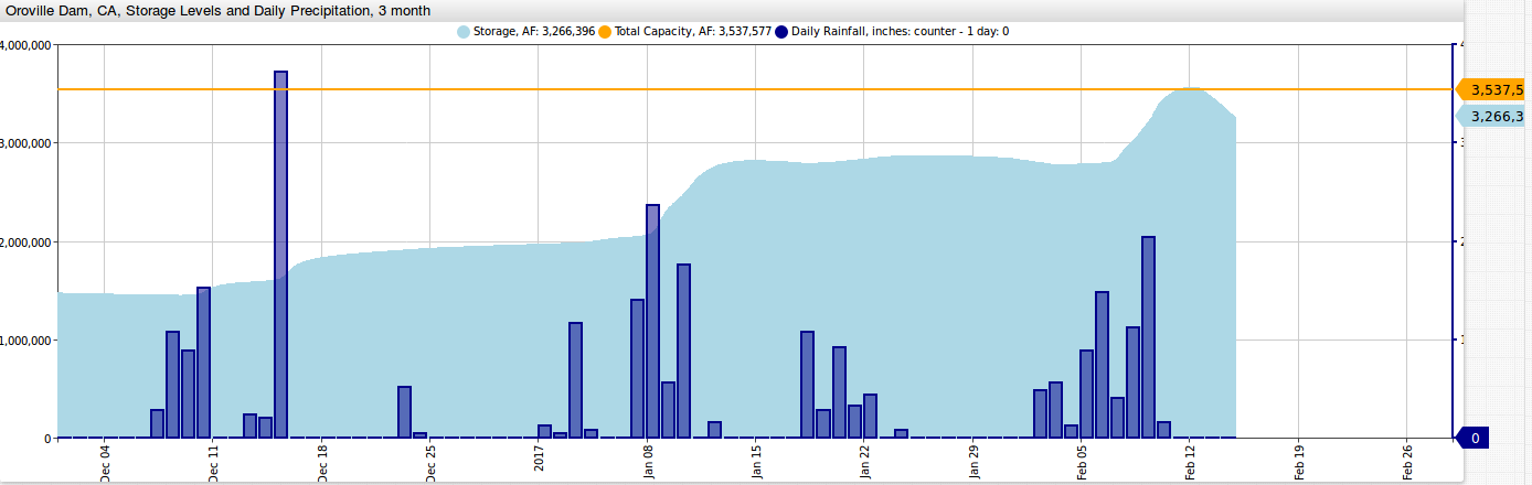
In the last several days, the storage level in the dam has dropped back down below the threshold capacity. The crisis, however, is not over quite yet. The main driving force behind the Oroville dam disaster has been a continued period of heavy rainfall in northern California. Below is an image showing daily precipitation totals together with the dam storage levels. By toggling over any of the columns, observe the values and time of these variables. After a period of rainfall, storage levels experience almost an immediate hike.

Below is a table of four of the most recent and significant rainfalls. Periods with rainfall accumulations over six inches led to massive increases in dam storage levels. Periods with rainfall accumulation less than 4 inches experienced much less drastic increases.

Rainfall Period	Accumulation (in)	Reservoir Storage Change (AF) (Values at 12:00 pm PT)	Net Change (AF)
Dec-07_Dec-10	3.8	1,468,037 (Dec-06) to 1,586,443 (Dec-12)	118,406
Jan-07_Jan-10	6.2	2,050,031 (Jan-06) to 2,830,139 (Jan-14)	780,108
Jan-18_Jan-22	3.0	2,811,974 (Jan-17) to 2,884,036 (Jan-25)	72,062
Feb-02_Feb-10	7.3	2,799,106 (Feb-05) to 3,578,686 (Feb-12)	779,580

You can explore this portal by clicking on the button below:

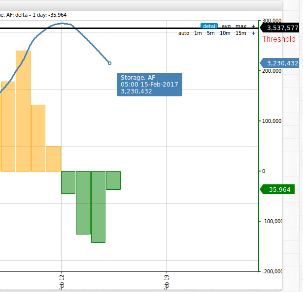
Below is an image of the situation at the time of publication. As of 5:00 am PT on February 15th, the reservoir storage level is at 3,230,432 AF, which is 307,145 AF less than the dam threshold. For the last several days, the storage level has been decreasing. However, rain has been forecast for the next several days.

Is there any way to predict how quickly the dam will fill up for a given amount of rainfall? Another helpful tool in ATSD is the capability to perform SQL queries, which can be used to search for specific information contained in this dataset. Using this query, obtain an estimate for the volume added (acre-foot) to the storage level of the reservoir per inch of rainfall.

SELECT
    SUM(t1.value)*3600*2.29569e-5 AS "total_inflow_in_acre_foot",
    DELTA(t2.value) AS "total_precipitation_inches",
    SUM(t1.value)*3600*2.29569e-5/DELTA(t2.value) AS "acre_foot_per_precipitation_inch"
FROM "ca.reservoir_inflow_cfs" t1
JOIN "ca.precipitation_accumulated_inches" t2
WHERE t1.datetime >= '2017-01-01T00:00:00Z'

| total_inflow_in_acre_foot  | total_precipitation_inches  | acre_foot_per_precipitation_inch |
|----------------------------|-----------------------------|----------------------------------|
| 2462228.8                  | 18.0                        | 136790.5                         |

Based off this estimate, for every inch of rainfall at the Oroville dam, 136,790.5 acre-feet are added to the reservoir. As of 5:00 am PT on February 15th, there is 307,145 AF of space left in the reservoir before it reaches its threshold. The maximum outflow per day that the dam is able is push out is 142,034 AFD, which was achieved on February 14th. Multiply the rainfall per day by the acre-feet rate (136,790.5) and subtract the maximum outflow, you get a storage amount added per day. If you then divide the storage added per day, you get an answer for how many days it would take for the storage to reach threshold capacity again. Below is a table showing the amount of time for the dam storage to reach threshold capacity for a given amount of rainfall per day.

Rainfall	Storage Added/Day	Remaining Storage	Time to Reach Threshold
1 inch per day	-5,243.5	307,145	No storage gain
2 inch per day	+131,547	307,145	2.334 days ~ 56 hours
3 inch per day	+268,337.5	307,145	1.144 days ~ 27 hours

Come back to these ChartLab portals in the coming days and look at the real-time analysis for updates on the Oroville dam. You do not need to install ATSD to continue to monitor the situation. Simply by clicking on each of the ChartLab buttons, you can keep up to date on dam storage levels, dam inflow, dam outflow, spillway outflow, and precipitation.

# Action Items

Below are the summarized steps to follow to install local configurations of ATSD and Axibase Collector for analyzing the Oroville dam disaster:

1. Install Docker.

2. Download the docker-compose.yml file to launch the ATSD Collector container bundle.

   curl -o docker-compose.yml https://raw.githubusercontent.com/axibase/atsd-use-cases/master/research/oroville-dam/resources/docker-compose.yml
   

3. In console, launch containers:

   export C_USER=username; export C_PASSWORD=password; docker-compose pull && docker-compose up -d
   

4. Import the cdec.water.ca.gov-shef-parser.xml file into ATSD. For a more detailed description, refer to step 9 from the following step-by-step walkthrough from the Axibase article describing U.S. mortality statistics.

5. Navigate to Axibase Collector main page https://docker_host:9443/ and manually run the following two imported docker-compose jobs: cdec.water.ca.gov-shef-daily and cdec.water.ca.gov-shef-hourly. You only need to run these jobs once, after which they run on a specified schedule.

6. Navigate to the ATSD Metrics page https://docker_host:8443/metrics and check that the metrics with the prefix ca. are in existence.