How To Calculate The Percentiles
Table of Contents
- How To Calculate The Percentiles
Terminology
Order Statistics
For a series of measurements X1, ..., XN, denote the data ordered in increasing order of magnitude by X(1), ..., X(N). These ordered data are called order statistics:
| i | Xi | X(i) |
|---|---|---|
| 1 | 50 | 10 |
| 2 | 40 | 12 |
| 3 | 40 | 14 |
| 4 | 30 | 16 |
| 5 | 20 | 18 |
| 6 | 18 | 20 |
| 7 | 16 | 30 |
| 8 | 14 | 40 |
| 9 | 12 | 40 |
| 10 | 10 | 50 |
The k-th order statistic is equal k-th smallest value. Special cases include:
- minimum:
X1 - maximum:
XN - range:
XN - X1 - midrange:
(XN - X1) × 1/2 - median: refer below
Rank
If X(j) is the order statistic that corresponds to the measurement Xi then the rank for Xi is j, i.e.
Ranking is the data transformation in which original values are replaced by their rank.
| i | Xi | X(i) | ri |
|---|---|---|---|
| 1 | 50 | 10 | 10 |
| 2 | 40 | 12 | 9 |
| 3 | 40 | 14 | 8 |
| 4 | 30 | 16 | 7 |
| 5 | 20 | 18 | 6 |
| 6 | 18 | 20 | 5 |
| 7 | 16 | 30 | 4 |
| 8 | 14 | 40 | 3 |
| 9 | 12 | 40 | 2 |
| 10 | 10 | 50 | 1 |
Percentiles
In Human Terms
Non-scientific definition:
the p-th percentile is a value below which a p% of observations fall.
In Scientific Terms
Below is the definition of percentile proposed by NIST Engineering Statistics Handbook:
the p-th percentile is a value, Pp, such that at most p% of the measurements are less than this value and at most (100−p)% are greater,
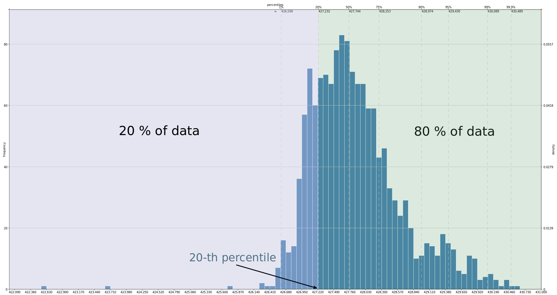
For the example above, in 20% of measurements the amount of available memory is less than 427.232, that means that P20=427.232.
Percentile Rank
A percentile rank is the proportion defined in percentile: for p-th percentile, rank is p. For instance, in the above example for 20-th percentile the rank is 20.
Quantile vs Percentile
It is more common in statistics to refer to quantiles. These are the same as percentiles, but are indexed by sample fractions rather than by sample percentages.
In general, the concepts of quantile and percentile are interchangeable, as well as the scales of probability calculation — absolute and percentage.
Statistics use the term q-quantiles. It stands for values that divide the order statistic into q subsets of equal sizes.
This means that the term percentiles is the name for 100-quantiles.
Also some other q-quantiles have special names:
decile ~ 10-quantile is any of the nine values that divide the order statistic into ten equal parts, and each part represents 1/10 of the sample or population.
median ~ 2-quantile is the value that divide the order statistic to the two equal parts.
quartile ~ 4-quantile is any of the three values that divide the order statistic to the four equal parts, named quarters.
The difference between upper and lower quartiles is also called the interquartile range → IQR = Q3 − Q1.
There are relations between different types of quantiles:
0 quartile = 0.00 quantile = 0 percentile

1 quartile = 0.25 quantile = 25 percentile

2 quartile = 0.50 quantile = 50 percentile = median

3 quartile = 0.75 quantile = 75 percentile

4 quartile = 1.00 quantile = 100 percentile
Estimation Of Percentiles
When there is a small sample of measurements, the CDF of the underlying population is unknown, that is why the percentile can not be calculated, it can be only estimated instead.
Often the percentile of interest is not correspond to a specific data point. In this case, interpolation between points is required. There is no a standard universally accepted way to perform this interpolation. Hyndman, R. J. and Fan, Y. (1986) described nine different methods for computing percentiles, most of statistical software use one of them.
Example Data
Consider these methods in the following example:
| i | Xi | X(i) |
|---|---|---|
| 1 | 50 | 10 |
| 2 | 40 | 12 |
| 3 | 40 | 14 |
| 4 | 30 | 16 |
| 5 | 20 | 18 |
| 6 | 18 | 20 |
| 7 | 16 | 30 |
| 8 | 14 | 40 |
| 9 | 12 | 40 |
| 10 | 10 | 50 |
N = 10
Notation:
q = p/100 - the percentile rank divided by 100
h - a computed real valued index
Xj - the j-th element of the order statistics, X3 = 16
⌈⌉ - ceil function, for example ⌈3.2⌉ = 4
⌊⌋ - floor function, for example ⌊3.2⌋ = 3
⌊⌉ - rounding to the nearest even integer, for example ⌊3.2⌉ = 4
Discontinuous Sample
R1. Inverse of EDF
h = N × qPp = X⌈h⌉if
q = 0,P0 = X1
| Percentile | Calculationsdata |
|---|---|
| 25-th | • h = 10 × 0.25 = 2.5 => ⌈h⌉ = ⌈2.5⌉ = 3• P25 = X3 = 14 |
The approach is used by1:
R2. Inverse of EDF with averaging at discontinuities
h = N × q + 1/2Pp = (X⌈h – 1/2⌉ + X⌊h + 1/2⌋) / 2if
q = 0,P0 = X1if
q = 1,P1 = XN
| Percentile | Calculationsdata |
|---|---|
| 25-th | • h = 10 × 0.25 + 0.5 = 3 => ⌈h – 1/2⌉ = ⌈2.5⌉ = 3, ⌊h + 1/2⌋ = ⌊3.5⌋ = 3• P25 = (X3 + X3) / 2 = 14 |
The approach is used by1:
R3. SAS definition: nearest even
h = N × qPp = X⌈h⌋if
q ≤ (1/2)/N,Pp = X1
| Percentile | Calculationsdata |
|---|---|
| 25-th | • h = 10 × 0.25 = 2.5 => ⌈h⌋ = 2• P25 = X2 = 12 |
The approach is used by1:
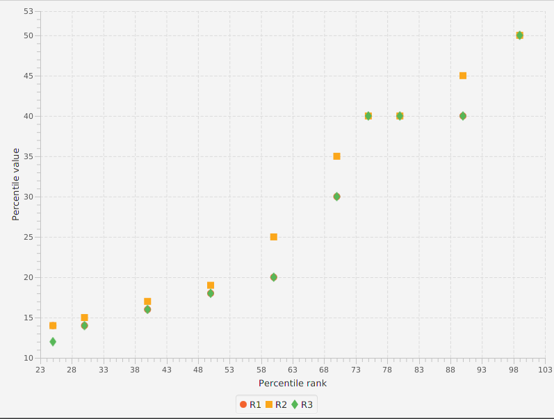
The graph below shows a comparison of the first three methods:
All subsequent methods use linear interpolation:
Pp = X⌊h⌋ + (h − ⌊h⌋) × (X⌊h⌋ + 1 - X⌊h⌋)
Continuous Sample
R4. Linear interpolation of the EDF
h = N × qPp = X⌊h⌋ + (h − ⌊h⌋) × (X⌊h⌋ + 1 - X⌊h⌋)if
q < 1/N,Pp = X1if
q = 1,P1 = XN
| Percentile | Calculationsdata |
|---|---|
| 25-th | • h = 10 × 0.25 = 2.5 => ⌊h⌋ = ⌊2⌋ = 2• P25 = X2 + (2.5 - 2) × (X3 - X2) = 13 |
The approach is used by1:
R5. Piecewise linear function
h = N × q + 1/2Pp = X⌊h⌋ + (h − ⌊h⌋) × (X⌊h⌋ + 1 - X⌊h⌋)if
q ≤ (1/2)/N,Pp = X1if
q ≥ (N - 1/2)/N,Pp = XN
| Percentile | Calculationsdata |
|---|---|
| 25-th | • h = 10 × 0.25 + 0.5 = 3 => ⌊h⌋ = ⌊3⌋ = 3• P25 = X3 + (3 - 3) × (X4 - X3) = 14 |
The approach is used by1:
*Note for the percentiles corresponding to the probabilities outside the range, prctile assigns the minimum or maximum values of the elements in X.
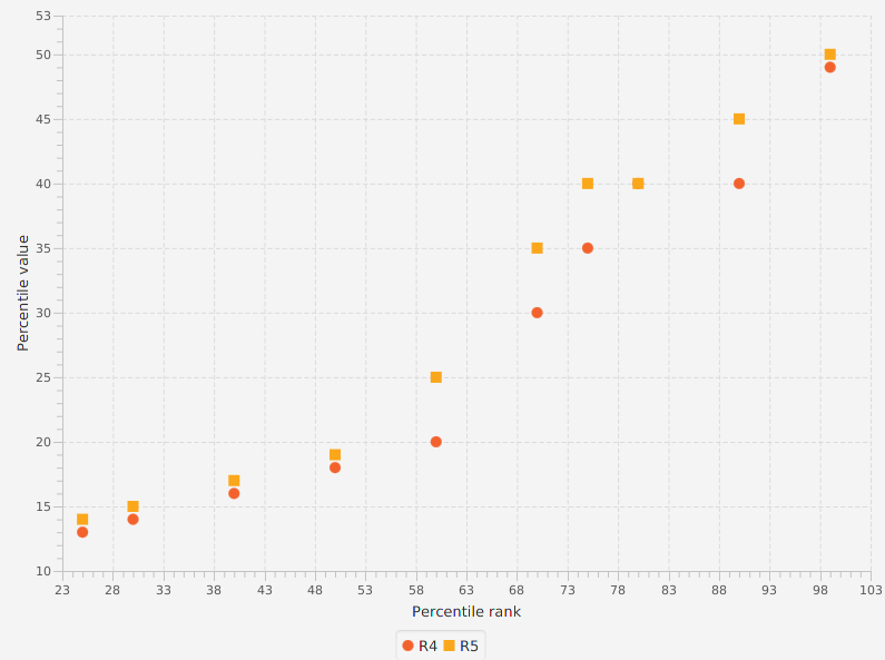
The graph below shows a comparison of the 4-th and 5-th methods:
R6. Linear interpolation of the mathematical expectations
h = (N + 1) × qPp = X⌊h⌋ + (h − ⌊h⌋) × (X⌊h⌋ + 1 - X⌊h⌋)if
q ≤ 1/(N + 1),Pp = X1if
q ≥ N/(N + 1),Pp = XN
| Percentile | Calculationsdata |
|---|---|
| 25-th | • h = (10 + 1) × 0.25 = 2.75 => ⌊h⌋ = ⌊2.75⌋ = 2• P25 = X2 + (2.75 - 2) × (X3 - X2) = 13.5 |
The approach is used by1:
- ATSD SQL PERCENTILE
- ATSD Rule Engine percentile()
- ATSD Data API PERCENTILE
- Charts PERCENTILE
- Excel PERCENTILE.EXC
- SAS
- SciPy v1.1.0
R7. Linear interpolation
h = (N - 1) × q + 1Pp = X⌊h⌋ + (h − ⌊h⌋) × (X⌊h⌋ + 1 - X⌊h⌋)if
q = 1,P1 = XN
| Percentile | Calculationsdata |
|---|---|
| 25-th | • h = (10 - 1) × 0.25 + 1 = 3.25 => ⌊h⌋ = ⌊3.25⌋ = 3• P25 = X3 + (3.25 - 3) × (X4 - X3) = 14.5 |
The approach is used by1:
- Excel PERCENTILE.INC
- Guava: Google Core Libraries for Java 23.0 API
- NumPy v1.15 with
interpolation : 'linear' - Pandas 0.23.4 with
interpolation : 'linear' - Oracle DB 10.2
This method is default in R.
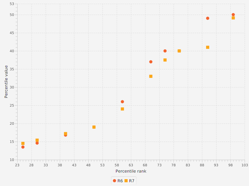
The graph below shows a comparison of the 6-th and 7-th methods:
R8. Linear interpolation of the approximate medians
The resulting quantile estimates are approximately median-unbiased regardless of the distribution of X.
The bias of an estimator is the difference between this estimator's expected value and the
truevalue of the parameter being estimated. An estimator or decision rule with zero bias is called unbiased. Otherwise the estimator is said to be biased.
h = (N + 1/3) × q + 1/3Pp = X⌊h⌋ + (h − ⌊h⌋) × (X⌊h⌋ + 1 - X⌊h⌋)if
q ≤ (2/3)/(N + 1/3),Pp = X1if
q ≥ (N - 1/3)/(N + 1/3),Pp = XN
| Percentile | Calculationsdata |
|---|---|
| 25-th | • h = (10 + 0.33) × 0.25 + 0.33 = 2.91 => ⌊h⌋ = ⌊2.91⌋ = 2• P25 = X2 + (2.91 - 2) × (X3 - X2) = 13.83 |
This method was recommended by Hyndman and Fan.
R9. Approximately unbiased estimates (if X is normally distributed)
h = (N + 1/4) × q + 3/8Pp = X⌊h⌋ + (h − ⌊h⌋) × (X⌊h⌋ + 1 - X⌊h⌋)if
q < (5/8)/(N + 1/4),Pp = X1if
q ≥ (N - 3/8)/(N + 1/4),Pp = XN
| Percentile | Calculationsdata |
|---|---|
| 25-th | • h = (10 + 0.25) × 0.25 + 0.375 = 2.93 => ⌊h⌋ = ⌊2.94⌋ = 2• P25 = X2 + (2.94 - 2) × (X3 - X2) = 13.875 |
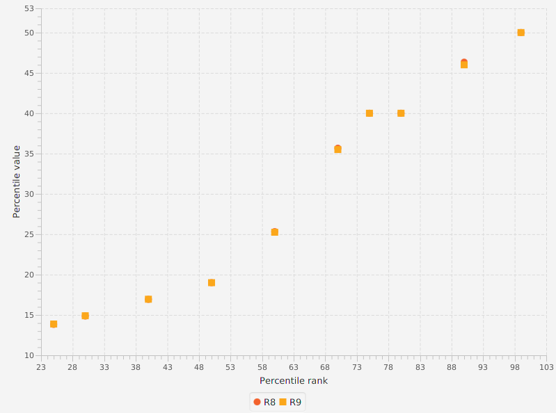
The graph below shows a comparison of the 6-th and 7-th methods:
Summaries
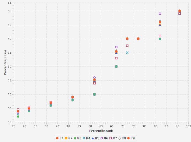
Key Percentiles Summary
| Percentile | R1 | R2 | R3 | R4 | R5 | R6 | R7 | R8 | R9 |
|---|---|---|---|---|---|---|---|---|---|
| 0 | 10 | 10 | 10 | 10 | 10 | 10 | 10 | 10 | 10 |
| 25 | 14 | 14 | 12 | 13 | 14 | 13.5 | 14.5 | 13.83 | 13.875 |
| 50 | 18 | 19 | 18 | 18 | 19 | 19 | 19 | 19 | 19 |
| 75 | 40 | 40 | 40 | 35 | 40 | 40 | 37.5 | 40 | 40 |
| 90 | 40 | 45 | 40 | 40 | 45 | 49 | 41 | 46.33 | 46 |
| 99 | 50 | 50 | 50 | 49 | 50 | 50 | 49.1 | 50 | 50 |
| 100 | 50 | 50 | 50 | 50 | 50 | 50 | 50 | 50 | 50 |
Methods Differences
| Method | Index h | Interpolation | Limits Selection |
|---|---|---|---|
| R1 | N × q | Pp = X⌈h⌉ | • q = 0 ⇒ P0 = X1 |
| R2 | N × q + 1/2 | Pp = (X⌈h – 1/2⌉ + X⌊h + 1/2⌋) / 2 | • q = 0 ⇒ P0 = X1• q = 1 ⇒ P1 = XN |
| R3 | N × q | Pp = X⌈h⌋ | • q ≤ (1/2)/N ⇒ Pp = X1 |
| R4 | N × q | X⌊h⌋ + (h − ⌊h⌋) × (X⌊h⌋ + 1 - X⌊h⌋) | • q < 1/N ⇒ Pp = X1• q = 1 ⇒ P1 = XN |
| R5 | N × q + 1/2 | X⌊h⌋ + (h − ⌊h⌋) × (X⌊h⌋ + 1 - X⌊h⌋) | • q ≤ (1/2)/N ⇒ Pp = X1• q ≥ (N - 1/2)/N ⇒ Pp = XN |
| R6 | (N + 1) × q | X⌊h⌋ + (h − ⌊h⌋) × (X⌊h⌋ + 1 - X⌊h⌋) | • q ≤ 1/(N + 1) ⇒ Pp = X1• q ≥ N/(N + 1) ⇒ Pp = XN |
| R7 | (N - 1) × q + 1 | X⌊h⌋ + (h − ⌊h⌋) × (X⌊h⌋ + 1 - X⌊h⌋) | • q = 1 ⇒ P1 = XN |
| R8 | (N + 1/3) × q + 1/3 | X⌊h⌋ + (h − ⌊h⌋) × (X⌊h⌋ + 1 - X⌊h⌋) | • q ≤ (2/3)/(N + 1/3) ⇒ Pp = X1• q ≥ (N - 1/3)/(N + 1/3) ⇒ Pp = XN |
| R9 | (N + 1/4) × q + 3/8 | X⌊h⌋ + (h − ⌊h⌋) × (X⌊h⌋ + 1 - X⌊h⌋) | • q < (5/8)/(N + 1/4) ⇒ Pp = X1• q ≥ (N - 3/8)/(N + 1/4) ⇒ Pp = XN |
Tools Summary
The following software provides functionality to use any of R1-R9:
qmust be in intervalq ∈ (0, 1], otherwiseorg.apache.commons.math3.exception.OutOfRangeExceptionis thrown.
NaN Strategy
-
Apache Commons Math 3.6 NaNStrategy:
MINIMAL - NaNs are treated as minimal in the ordering, equivalent to (that is, tied with) Double.NEGATIVE_INFINITY MAXIMAL - NaNs are treated as maximal in the ordering, equivalent to Double.POSITIVE_INFINITY REMOVED - NaNs are removed before the rank transform is applied FIXED - NaNs are left "in place," that is the rank transformation is applied to the other elements in the input array, but the NaN elements are returned unchanged. FAILED - If any NaN is encountered in the input array, an appropriate exception is thrown. -
na.rm - if true, any NA and NaN's are removed from x before the quantiles are computed
if false NA and NaN values are not allowed
ATSD
NaN values are removed before the percentiles are estimated.
Graphical Representation Of Percentiles
Box-And-Whiskers Diagram or Box Plot is the visual representation of the several percentiles of a given data set.
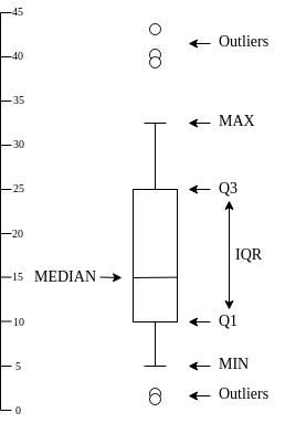
Outliers are described below.
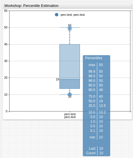
Below is the Box Plot for the example data.
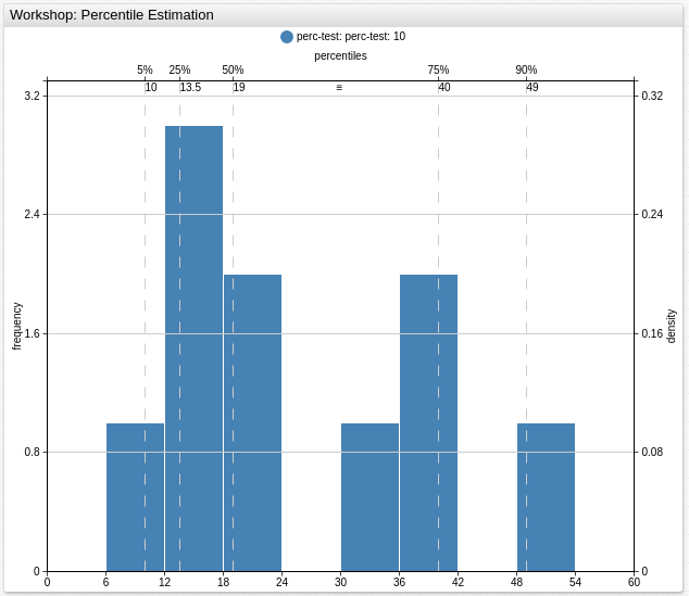
It is also convenient to display the percentiles in the Histogram Chart.
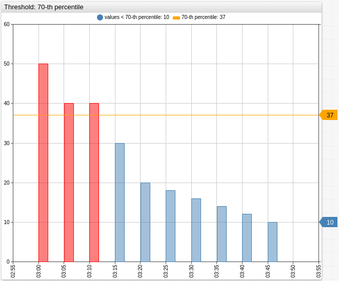
Percentiles are often used for thresholds checking, below values that are greater than P70 = 37 are colored in red.
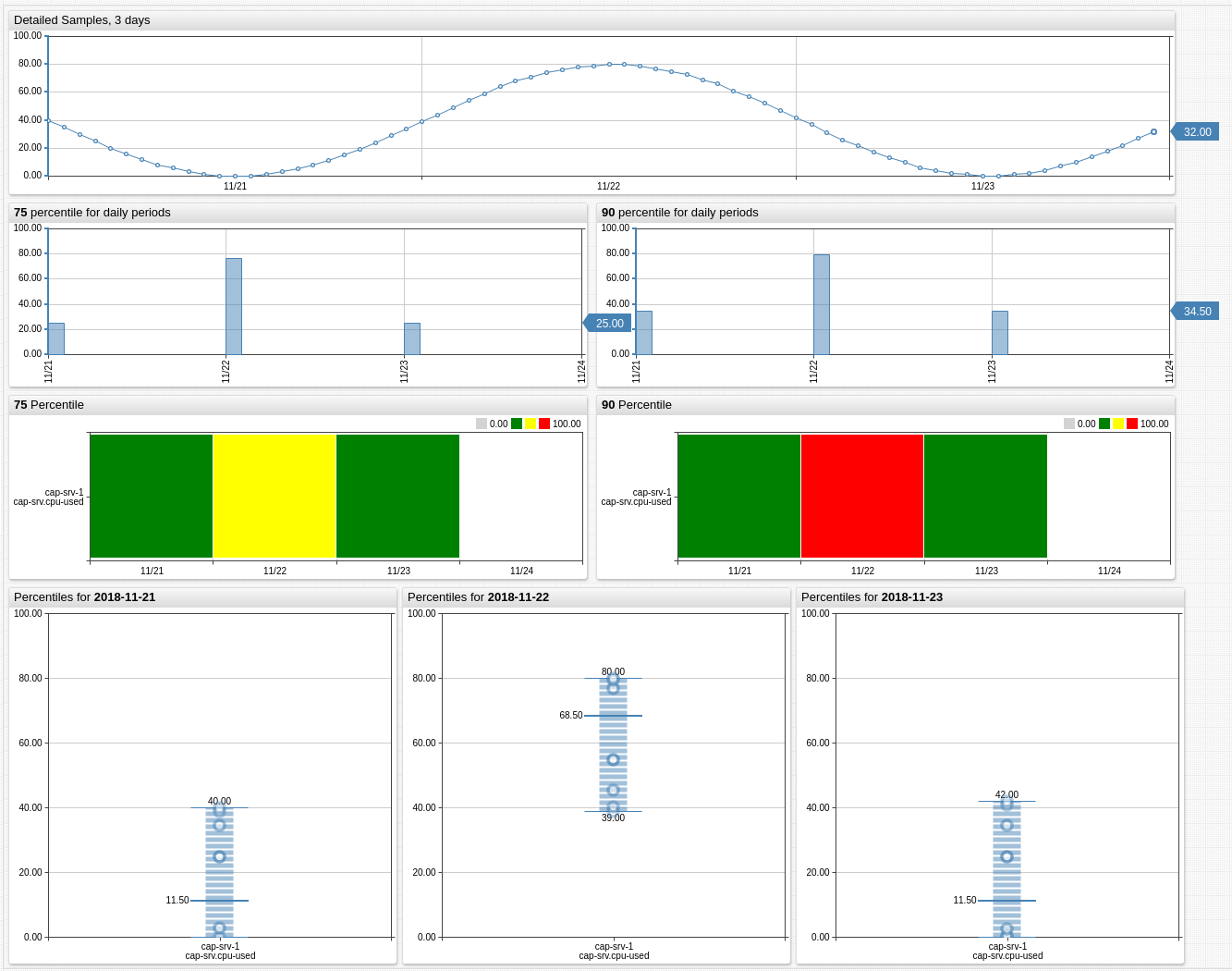
Additional Examples
Robust Statistics
The term "robust statistics" is closely related to the term "outliers".
Outlier is an observation (or subset of observations) which appears to be inconsistent with the remainder of that set of data.
This definition is not precise, the decision whether an observation is an outlier, is left to the subjective judgement of the researcher.
Robust statistics are resistant to outliers. In other words, if data set contains very high or very low values, then some statistics will be good estimators for population parameters, and some statistics will be poor estimators. For example, the arithmetic mean is very susceptible to outliers (it is non-robust), while the median is not affected by outliers (it is robust).
Median vs Average
Average or arithmetic mean is the sum of the numbers divided by how many numbers are being averaged:
The median is a robust measure of central tendency, while the mean is not.
For the symmetric distributions (normal in particular) the mean is also the median.
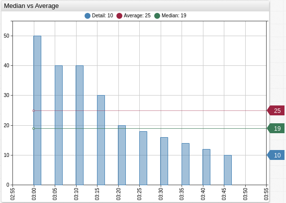
For the example sample mean is greater than median:
Median Absolute Deviation vs IQR vs Standard Deviation
Median Absolute Deviation, IQR and Standard Deviation are measures of spread (also called measures of dispersion), that means that they show something about how wide the set of data is.
The standard deviation is a measure of how spread out data is around center of the distribution. It also gives an idea of where, percentage wise, a certain value falls.
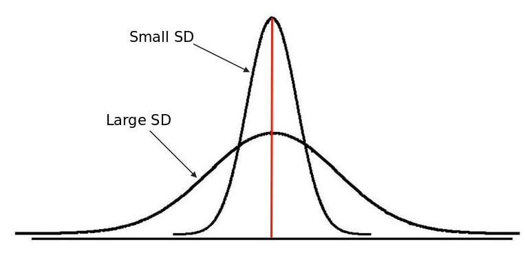
The SD is affected by extremely high or extremely low values and non normality, in other words it is not robust.
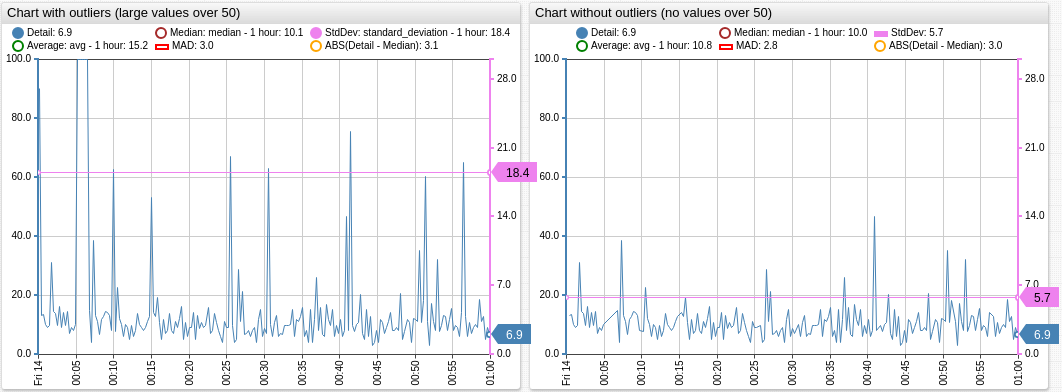
The median absolute deviation is a robust measure of how spread out a set of data is.
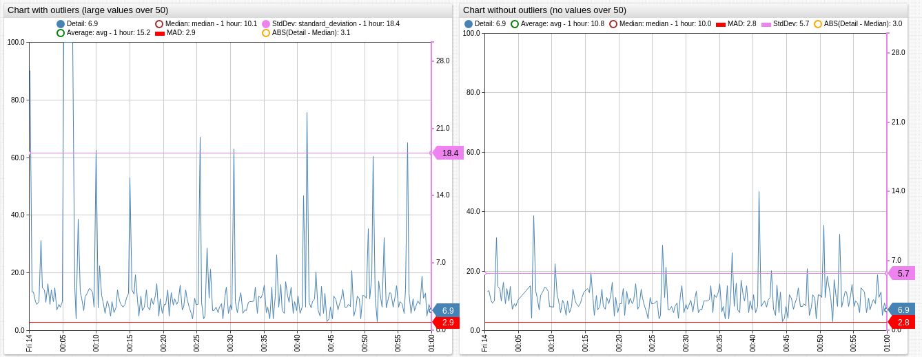
If data is normally distributed, the SD is usually the best choice for assessing spread, otherwise, the MAD is preferred, but it must be multiplied with scale factor k - a constant linked to the assumption of normality of the data, read additional information in [3] and [6].
The IQR is similar to the MAD, but it is less robust.
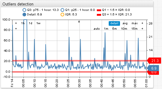
The IQR is often used to find outliers in sample: observations that fall below Q1 − 1.5 × IQR or above Q3 + 1.5 × IQR are marked as outliers. In a box plot, the highest and lowest occurring value within this limit are indicated by whiskers of the box and any outliers as individual points.
IQR can also be used as a threshold.
Sources
- "A Brief Introduction to Robust Statistics", André Lucas
- Apache Commons Math 3.6 Percentile
- "Detecting outliers: Do not use standard deviation around the mean, use absolute deviation around the median", Leys, C., Journal of Experimental Social Psychology (2013)
- "Introduction to Statistics", Stepik course
- NIST Engineering Statistics Handbook
- R mad
- R quantile
- "Statistical Computing", Hyndman, R. J. and Fan, Y. (1986)
- Statistics How To
- Wolfram MathWorld Order Statistic
- Wiki Quantile

