What is Docker and How Do You Monitor It?

What is Docker and How Do You Monitor It?

In recent months Docker has become the hot topic in Server Infrastructure and DevOps conversations. It seems like everyone is either deploying on Docker, integrating with Docker, or developing for Docker. It’s an understandable position: Linux containers provide a lot of benefits for developers while allowing the operations team to manage their infrastructure as a homogeneous pool of computing resources, as opposed to siloed, host-based installations.

Summary

Are you already familiar with Docker and Linux containers? Would you like to monitor containerized services for availability and performance without resorting to legacy approaches such as using host naming conventions or scheduled CMDB discovery?

We recommend adopting a policy of assigning container labels so that your services can be monitored based on a combination of built-time and run-time metadata.

Leverage the fact that container labels override image labels by delegating labeling responsibilities to operations and development teams.

For build-time metadata, collaborate with developers to ensure that Dockerfiles include labels classifying images with service, application, product, function, and versioning information.

FROM ubuntu:14.04
MAINTAINER ATSD Developers <dev-atsd@axibase.com>
ENV version 12.1.2
 
#metadata
LABEL com.axibase.vendor="Axibase Corporation" \
  com.axibase.product="Axibase Time Series Database" \
  com.axibase.code="ATSD" \
  com.axibase.function="database" \
  com.axibase.revision="${version}"</dev-atsd@axibase.com>

See ATSD Dockerfile as an example.

On the operating side, assign runtime labels when starting containers:

docker run \
  --detach \
  --name=atsd \
  --publish 8443:8443 \
  --label=com.axibase.service=metrics \
  --label=com.axibase.business-unit=monitoring \
  --label=com.axibase.region=us-east-1 \
  --label=com.axibase.zone=us-east-1b \
  --label=com.axibase.environment=production \
  axibase/atsd:latest

Whether or not container labels are assigned manually, using deployment scripts, or through orchestration frameworks such as Kubernetes or Mesos that manage containers on a large fleet of machines is an implementation detail that is specific to each organization.

Once you have container labeling in place, you can create roll-up dashboards and configure alerting without referring to hostnames or container ids/aliases.

Instead, containers can be grouped and filtered based on their labels (tags in ATSD terms) using expressions. For example:

tags['com.axibase.service'] == 'metrics' && tags['com.axibase.environment'] == 'production'

This expression will group all containers that support metrics service in production. New containers will be automatically added to the roll-up. When a container is terminated, it will not be removed from the group, allowing you to see detailed historical data for the selected service.

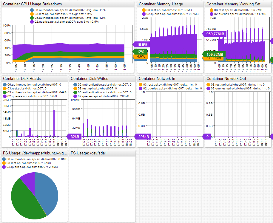
Grouping based on metadata allows you to build roll-up portals. Below is an example of a portal for API service containers running in the SVL datacenter. We can see the API service broken down by container, which gives us insight into the overall service performance and the performance of individual micro-services.

See deployment instructions here.

What is Docker?

The Docker set of tools includes a runtime engine for managing containers, a layered file-system format, and a publicly hosted registry of images for widely used off-the-shelf applications. In basic terms, the Docker engine provides automation for the deployment of applications inside Linux containers.

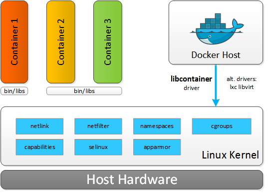
Resource isolation features of the Linux kernel, such as cgroups, namespaces, and chroot, allow groups of processes to have a private view of the system and run independently on a single Linux host. This architecture lets you avoid the overhead of starting and running several virtual machines (VMs). Since VMs run on a Host OS, each new application needs to start a Guest OS. This process doesn’t scale well for micro-service architectures, where the footprint of services is smaller but at the same time their count is greater. In Docker, you simply start applications as a group of processes that remain separate from one another while sharing underlying computing resources.

When comparing Linux containers with virtual machines, VMs require more resources but provide better isolation since VM hypervisors emulate the full operating system stack including virtual hardware. Containers, on the other hand, run on a shared operating system. Containers leave most of the VM bulk behind (VM sizes can often reach tens of gigabytes) in favor of a miniature package that contains the application and its dependencies. As a result, a Docker host can run many more applications on identical hardware.

What Are Linux Containers?

Containers are wrapped-up applications and pieces of software that include all dependencies but use a shared kernel with other containers (applications). Essentially, containers are isolated sets of processes in the userspace on the host operating system. While Hypervisors abstract the entire device, containers just abstract the operating system kernel. One important limitation is the fact that all containers running on a single machine must use the same kernel (Host OS), whereas with Hypervisors each VM can run its own Guest OS with different kernels.

Another key difference between containers and VMs is execution speed. Launching a VM can take several minutes and is often very resource intensive. So, launching several VMs requires some planning and scheduling. You can launch multiple containers within seconds, as they are very lightweight. This kind of performance and scalability leads to a new type, maybe even a new generation, of distributed applications where containers are automatically launching and stopping depending on various factors like user traffic, events, queries, scheduled tasks, etc.

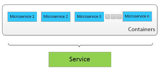
Micro-services and the Right Approach to Collecting Docker Performance Data

Executing containers on Docker enables decomposition of applications into micro-services which improves fault tolerance and manageability. However, the side effect is more challenging performance monitoring, since micro-service life cycles can be very short. The lifespan of containers can be as short as just a few minutes – in some cases even seconds – while Virtual Machines can have lifespans measured in years. So while treating containers like VMs might seem convenient, it is a misleading analogy.

Container statistics are often gathered for a short timespan, meaning that traditional ways of monitoring are not applicable. Once the container is terminated, its data becomes obsolete for the purpose of troubleshooting, since its workload has been taken over by a new container. Instead of chasing individual container identifiers, consider monitoring applications and services based on labels: application name, type, role, function etc. This can be accomplished by leveraging container labels to encode type, role, or function groups. In order to provide a meaningful amount of metadata about each micro-service, container labels should include:

• service/application name
• function such as database, message-broker, http-server
• environment such as testing, staging, production
• datacenter topology: dc name, region, availability zone

When such a naming convention is enforced, monitoring and alerting tools can visualize and prioritize data based on predefined labels. For example, you can easily report on:

• Average CPU utilization for containers that are part of the specified service name
• Number of logins for micro-services that execute the authentication function for web applications
• Total memory allocated and used by containers that are part of API applications hosted in a particular datacenter

The more metadata we have about each container, the easier it is to aggregate relevant information. With this approach you won’t be looking at statistics from terminated containers. Moreover, you will see exactly what is happening at the micro-service, service, or application level. You can look at the big picture or drill down to the smallest details.

Allocating Resources

Allocation of resources to containers is especially important as containers are less isolated than virtual machines. A single runaway container can lead to performance issues and degradation across the entire host. In Hypervisors, VMs are normally allocated a fixed amount of CPU resources, RAM, and disk space, meaning that the applications will work within those set limits regardless of the load to which the VM or application is subjected.

CPU

Each container is assigned a “share” of the CPU, set to 1024 by default. By itself, 1024 CPU share does not mean anything. If there is only a single container running, then it can use all the available CPU resources. However, if you launch another container and both containers have 1024 CPU share, then each container can claim only 50% of the total available CPU resources.

CPU share is set using the -c or --cpu-shares flag when launching the container.

For example:

docker run -ti -c 1024 ubuntu:14.04 /bin/bash

Suppose there are three containers running — two with 1024 CPU share and one with 512. This will mean that the two containers with 1024 CPU share can each use 40% of the CPU, while the container with the 512 CPU share will be limited to 20%. The logic here is that we take the total number of shares the CPU currently has and split them up like corporate stock. If you have half of all the shares, then you get 50% of the voting rights. The same principle applies here to container CPU usage.

This scenario is only true for hosts operating under load where CPU resources are scarce. On an idle system running multiple containers, a single container with a small CPU share will be able to utilize 100% of the unused CPU capacity.

Another option for setting CPU limits is CPU CFS. In this case, we are setting CPU Period (100ms by default) and CPU Quota (number of cpu ticks allocated to a container).

For example:

docker run -ti --cpu-period=50000 --cpu-quota=10000 ubuntu:14.04 /bin/bash

This would result in the container getting 20% of the CPU run time every 50 ms. This is a stricter limit than when setting CPU shares, since in this case the container is not able to surpass the set limit on an idle system.

Containers can also be assigned to use only specific CPUs or CPU cores. In this case, the CPU share system only applies to processes running on the same core. If you have two containers that are assigned to different CPU cores (assuming that there are no other containers running), then both of these containers will be able to utilize 100% of their CPU core regardless of the shares. That is, until other containers are launched or assigned to these CPU cores.

Memory

Things are more simple when it comes to memory. Memory can be limited with a short command (-m flag) and the limits are applied to both memory and swap.

For example:

docker run -ti -m 300M --memory-swap 300M ubuntu:14.04 /bin/bash

This sample command will limit the container memory and swap space usage to 300MB each.

Currently, it is not possible to separately control the amount of allocated memory and swap in Docker. Hopefully, this will change in the future. By default, when a container is launched, there are no set memory limits. This can lead to a single container using all the memory and making the entire system unstable.

Disk

Disk space and read/write speed can be limited in Docker. By default, read/write speed is unlimited. However, if required, it can be limited as needed using the io controller in cgroups.

In conclusion, controlling resource allocation is easy, so you should use it. Resource management should be controlled automatically based on the container type, application, and micro-service that is being launched. In production deployments, resource allocation should be planned well ahead of time and done automatically, as it’s becoming the norm to constantly launch and stop containers depending on various events and factors. The bottom line is that managing resources by hand in production environments is simply out of question.

Collected Docker Metrics

Currently, there are a variety of metrics collected by Docker. They are broken down into several categories: CPU, memory, I/O, and network. A complete list of collected metrics can be found at the bottom of this page.

Docker Monitoring Scenarios

The main point of monitoring Docker performance is to maximize the efficiency of your hardware. You don’t want those expensive machines and cloud infrastructure standing idle and you definitely don’t want your hosts being unusable due to the load of resource-starved containers. The goal is to maximize the load of your infrastructure without sacrificing performance of any applications or micro-services.

The collected Docker metrics can be used to automate a large part of the capacity planning.

Resource-Aware Scheduling and Auto-scaling

This type of implementation will:

• start new containers on machines where the load is lower
• stop containers on machines where performance thresholds are being reached

This type of implementation will be constantly stopping, starting, and migrating containers inside the infrastructure. That will ensure that all containers have the resources they need and that all the machines are running at the most efficient capacity. Automation of this magnitude must be based on advanced machine learning algorithms and forecasts. The automated system also must have the capability to make its own decisions based on its analysis of the system performance metrics.

In complex infrastructures, a single resource-starved micro-service can lead to a chain reaction across the whole application. Automating capacity planning is key for managing large numbers of Linux containers.

Automated Monitoring and Alerting

Of course machines and systems fail if thresholds are breached or forecasts/trends are negative. In that case, container owners should be immediately alerted of performance issues.

In order for these alerts to be raised and delivered proactively (using system performance forecasting and trending methods), an automated thresholding and alerting system must be in place. The Axibase Time Series Database Rule Engine combined with built-in Forecasting tools are capable of resolving this issue autonomously.

The Rule Engine applies statistical functions to incoming data streams before the data is stored on disk. In the Rule Engine, you can create alerting rules with time-/count-based sliding windows, aggregation, and forecasting functions. Raised alerts can be delivered to enterprise consoles, email, and ticketing systems. System commands can be executed automatically based on alert-action settings.

In other words, the Rule Engine can monitor a wide collection of metrics based on a set of “smart rules.” It will raise alerts and inform the container owners of performance issues. Further, the Rule Engine is capable of executing system commands to potentially start or stop containers or modify certain settings.

The Rule Engine works based on machine learning algorithms. Together with advanced Holt-Winters and ARIMA forecasting functions, it enables so-called “predictive maintenance” when the system forecasts issues before they occur based on negative trends and historical data. This gives you valuable time to navigate the rough patches and prevents you from having to revive a crashed system.

Here is how some of our customers use ATSD to monitor their Linux containers:

Most customers almost completely eliminate base thresholds from their alerting catalog in favor of automated thresholds and dynamic rules.

Here are a few sample rules applied to various metrics:

abs(avg() - forecast()) > 25

This rule will raise an alert if the absolute forecast deviates from the 5-minute average by more than 25.

abs(forecast_deviation(wavg())) > 2

This rule will raise an alert if the absolute forecast deviates from the 15-minute weighted average by more than 2 standard deviations.

avg(value) / avg(value(time: '1 hour')) > 1.25

This rule will raise an alert if the 15-minute average exceeds the 1-hour average by more than 25%.

These rules adapt to events and change over time. If your daily number of users is growing, so is the load. This rule will take that fact into account when calculating thresholds. This is where daily re-calculation of forecasts in ATSD shows its strengths – it allows ATSD to determine new periods and new trends continuously. New forecasts are generated every night, taking into account all the recent developments and trends that have occurred. This kind of approach results in improved forecast accuracy and dynamic response to abnormal events and new trends.

As a result of “smart rules” and advanced forecasting techniques, you are able to leave alerting and monitoring tasks in the capable hands of ATSD. The Axibase Time Series Database will inform you of critical events and negative forecasts. In addition, it will eliminate the need to revisit and adapt thresholds manually, which can be a time-consuming task in itself. In short, automated thresholding is the future of performance monitoring.

Monitoring Linux Containers with the Axibase Time Series Database

Modern companies are becoming increasingly overwhelmed with machine data. They can rarely leverage this information to predict operational behavior of their systems, applications, and users because advanced analytics and forecasts require detailed data collected for several business cycles (years) to be accurate. ATSD solves this problem by storing granular data for long periods of time in order to support fully automated, adaptive thresholding at scale.

ATSD allows you to:

• Store detailed operational metrics for years without precision loss
• Datamine these metrics to predict problems and uncover hidden opportunities
• Improve precision of capacity planning and performance monitoring

Axibase is focused on three crucial points with respect to performance monitoring:

• Visibility
• Control
• Automation.

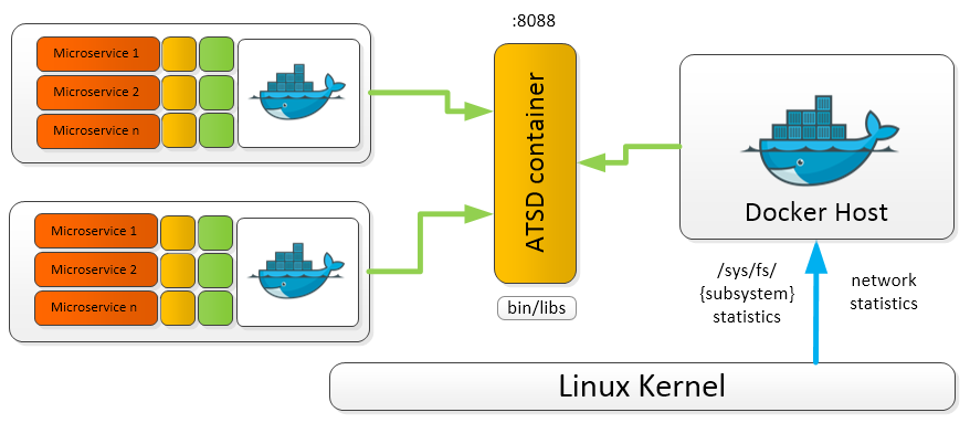
The Axibase Time Series Database can collect Docker metrics for long-term retention, analytics, and visualization. A single ATSD instance can collect metrics from many Docker hosts.

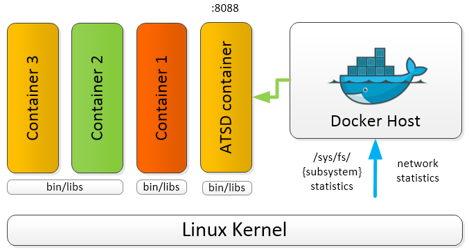
ATSD stores metrics from local and remote Docker hosts for consolidated monitoring and analytics. This way, it serves as a single point of access for performance monitoring and capacity planning.

On top of the data that ATSD retrieves from Docker, we recommend that you install scollector, tcollector, collectd, or nmon for a more in-depth look into system performance.

To get started with Docker monitoring, continue reading ATSD setup and usage guides here.

Collected Metrics

Complete list of metrics collected by Axibase Time Series Database:

CPU

cpu.loadaverage
cpu.usage.percpu
cpu.usage.percpu%
cpu.usage.system
cpu.usage.system%
cpu.usage.total
cpu.usage.total%
cpu.usage.user
cpu.usage.user%

I/O

diskio.ioservicebytes.async
diskio.ioservicebytes.read
diskio.ioservicebytes.sync
diskio.ioservicebytes.total
diskio.ioservicebytes.write
diskio.ioserviced.async
diskio.ioserviced.read
diskio.ioserviced.sync
diskio.ioserviced.total
diskio.ioserviced.write
taskstats.nriowait
taskstats.nrrunning
taskstats.nrsleeping
taskstats.nrstopped
taskstats.nruninterruptible

Memory

memory.containerdata.pgfault
memory.containerdata.pgmajfault
memory.hierarchicaldata.pgfault
memory.hierarchicaldata.pgmajfault
memory.usage
memory.workingset

Network

network.rxbytes
network.rxdropped
network.rxerrors
network.rxpackets
network.txbytes
network.txdropped
network.txerrors
network.txpackets