Stata

Prerequisites
Loading Data
Exporting Data
Calculating Derived Series
Reference

Prerequisites

Install Stata 15
Install ODBC-JDBC Bridge

If your ATSD installation has too many metrics (more than 10000), add a tables={filter} parameter to the JDBC URL to filter the list of tables visible in Stata.

Loading Data

Set encoding for the ODBC Driver in the Stata console: set odbcdriver ansi

This configures Stata to interface with ODBC in ANSI mode to prevent string values from being truncated.

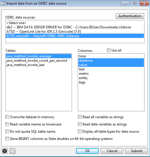
Load Data using Import Wizard

Click File > Import > ODBC data sources
Select the ATSD connection in ODBC data sources
Select a table in the Tables list
Choose one or multiple columns from the Columns list
Click OK to import rows containing data in these columns into Stata memory

Load Data with Stata Console

Type odbc list in the Stata Console.
Click the ATSD Data Source Name (DSN) that you have configured in the ODBC-JDBC Bridge

Click a table from the list to view the table description:

Click load to load the entire table as a dataset into memory.
Click query to re-load the list of tables.

Load Data with SQL Query

Execute odbc load to load results for a custom SQL query results into memory:

odbc load, exec("SELECT time, value, tags.name FROM java_method_invoke_last ORDER BY datetime LIMIT 100") bigintasdouble

Syntax:

exec("SqlStmt") allows to issue an SQL SELECT statement to generate a table to be read into Stata.
bigintasdouble specifies that data stored in 64-bit integer (BIGINT) database columns be converted to Stata doubles.

Description of result set:

Convert Unix Time Milliseconds to Stata Milliseconds

generate double datetime = time + tC(01jan1970 00:00:00)
format %tcCCYY-NN-DD!THH:MM:SS.sss!Z datetime

Description of result set:

Exporting Data

Export Data using Export Wizard

Follow the path File > Export > ODBC data source.
Click the ATSD connection in ODBC data sources.
Type the table name into Tables field. This is the metric name holding the exported data.
Choose the variables to export in the Variables drop-down list.
Type column names from the target metric according to variables selected in the previous step.
Choose Append data into existing table in Insertion options.
Check Use block inserts option.
Click OK to export the selected variables into ATSD.

Export Data using Stata Console

Use the odbc insert command to write data from Stata memory into ATSD.

odbc insert var1 var2 var3, as("entity datetime value") dsn("ATSD") table("target_metric_name") block

Enable the block setting to insert all available records.

Syntax:

var1 var2 var3 is a list of variables from the in-memory dataset in Stata.
as("entity datetime value") is a list of columns in the ATSD metric. It is sorted according to list of variables.
dsn("ATSD") is a name of ODBC connection to ATSD.
table("metric_name") is a name of the metric which contains exported dataset.
block is a parameter to force using block inserts.

Calculating Derived Series

To calculate the category-weighted consumer price index (CPI) for each year, the CPI value for a given category must be multiplied by its weight and divided by 1000 since its weights are stored as units of 1000 (not 100). The resulting products are summed as the weighted CPI for the given year.

Load and Save Prices

odbc load, exec("SELECT value as price, tags.category as category, datetime FROM inflation.cpi.categories.price ORDER BY datetime, category") dsn("ODBC_JDBC_SAMPLE")
save prices

The data is saved for later access.

Preview prices:

prices dataset description:

Load and Save `Datetimes`

clear
odbc load, exec("SELECT datetime FROM inflation.cpi.categories.price GROUP BY datetime ORDER BY datetime") dsn("ODBC_JDBC_SAMPLE")
save datetimes

Preview datetimes dataset:

Load Category Weights

clear
odbc load, exec("SELECT tags.category as category, value as weight FROM inflation.cpi.categories.weight ORDER BY datetime, category") dsn("ODBC_JDBC_SAMPLE")

Since the Weights are available for only one year, assume that the category weights are constant through the timespan and therefore can be repeated for each year from 2013 to 2017.

Perform a cross join of weights with datetimes:

cross using datetimes

Preview the joined dataset:

Merge Weights with Prices

In this step two tables are appended to perform calculations within one table. This table has a unique row identifier (composite key of datetime + category) to join rows with the INNER JOIN operation.

merge 1:1 category datetime using prices
drop category _merge

Preview the merged dataset:

Calculate New Variable

Multiply two columns element-wise to calculate the inflation index per category:

generate inflation = weight * price / 1000
drop weight price

Preview the dataset:

Group Rows by Date and Aggregate SUM

Group rows by datetime and sum weighted price values for each year.

bysort datetime : egen value = total(inflation)
sort datetime value
by datetime value :  gen dup = cond(_N==1,0,_n)
drop if dup>1
drop dup inflation

This operation groups records by datetime and calculate the sum of the inflation values for each group.

Preview the dataset:

Add Entity Constant

The entity column is required to store the calculated variable in ATSD.

generate entity = "bls.gov"

This operation adds a new column entity with value bls.gov in each row.

Preview the dataset:

Insert Data into ATSD

Result set description:

`datetime` as NUMBER

replace datetime = datetime - tC(01jan1970 00:00:00)
set odbcdriver ansi
odbc insert entity datetime value, as("entity datetime value") table("inflation.cpi.composite.price") dsn("ODBC_JDBC_SAMPLE") block

`datetime` as STRING

generate datetime_str = string(datetime, "%tcCCYY-NN-DD!THH:MM:SS.sss!Z")
set odbcdriver ansi
odbc insert entity datetime_str value, as("entity datetime value") table("inflation.cpi.composite.price") dsn("ODBC_JDBC_SAMPLE") block

Check Results

SELECT entity, datetime, value FROM inflation.cpi.composite.price

| entity  | datetime                 | value              |
|---------|--------------------------|--------------------|
| bls.gov | 2013-01-01T00:00:00.000Z | 100.89632897771745 |
| bls.gov | 2014-01-01T00:00:00.000Z | 101.29925299205442 |
| bls.gov | 2015-01-01T00:00:00.000Z | 100.60762066801131 |
| bls.gov | 2016-01-01T00:00:00.000Z | 100.00753061641115 |
| bls.gov | 2017-01-01T00:00:00.000Z | 100.12572021999999 |

Script File

Link to the do file that contains the recorded transformations.

Reference

Stata commands used in this example:

# Stata

# Prerequisites

# Loading Data

# Load Data using Import Wizard

# Load Data with Stata Console

# Load Data with SQL Query

# Convert Unix Time Milliseconds to Stata Milliseconds

# Exporting Data

# Export Data using Export Wizard

# Export Data using Stata Console

# Calculating Derived Series

# Load and Save Prices

# Load and Save Datetimes

# Load Category Weights

# Merge Weights with Prices

# Calculate New Variable

# Group Rows by Date and Aggregate SUM

# Add Entity Constant

# Insert Data into ATSD

# datetime as NUMBER

# datetime as STRING

# Check Results

# Script File

# Reference

Stata

Prerequisites

Loading Data

Load Data using Import Wizard

Load Data with Stata Console

Load Data with SQL Query

Convert Unix Time Milliseconds to Stata Milliseconds

Exporting Data

Export Data using Export Wizard

Export Data using Stata Console

Calculating Derived Series

Load and Save Prices

Load and Save `Datetimes`

Load Category Weights

Merge Weights with Prices

Calculate New Variable

Group Rows by Date and Aggregate SUM

Add Entity Constant

Insert Data into ATSD

`datetime` as NUMBER

`datetime` as STRING

Check Results

Script File

Reference